
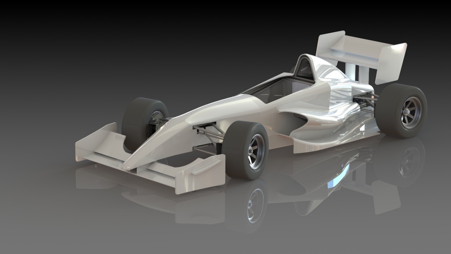
A wider wing can produce more downforce, but it can also reduce maximum speed. A smaller wing can reduce drag, but the loss of grip may cost time through corners. Choosing the right shape means understanding how these effects work together.
At McCarbon, we use computational fluid dynamics, or CFD, to investigate these choices. CFD calculates airflow around a digital vehicle. It predicts the forces produced by that airflow and shows where they act.
We can then combine these results with information about the engine, gearbox, tyres and vehicle mass to estimate their effect on the whole car.
What can we change, and why?
Wing angle, width and profile are useful starting points. The profile is the curved shape seen when a wing is viewed in cross-section. Changing it alters how air passes around the wing and the pressure acting on its surfaces.
We can also change individual wing elements, their position, or whether they are fitted at all. These adjustments help us investigate how much downforce a component provides and how much drag it adds.
The geometry before simulation
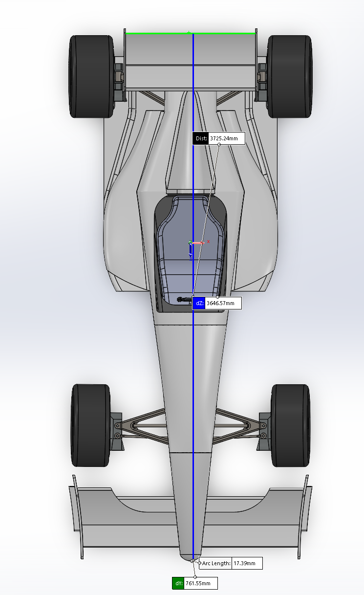
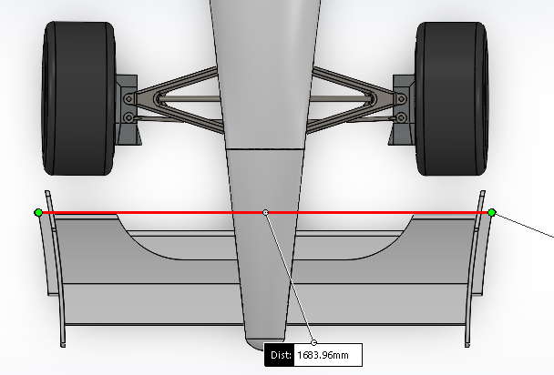
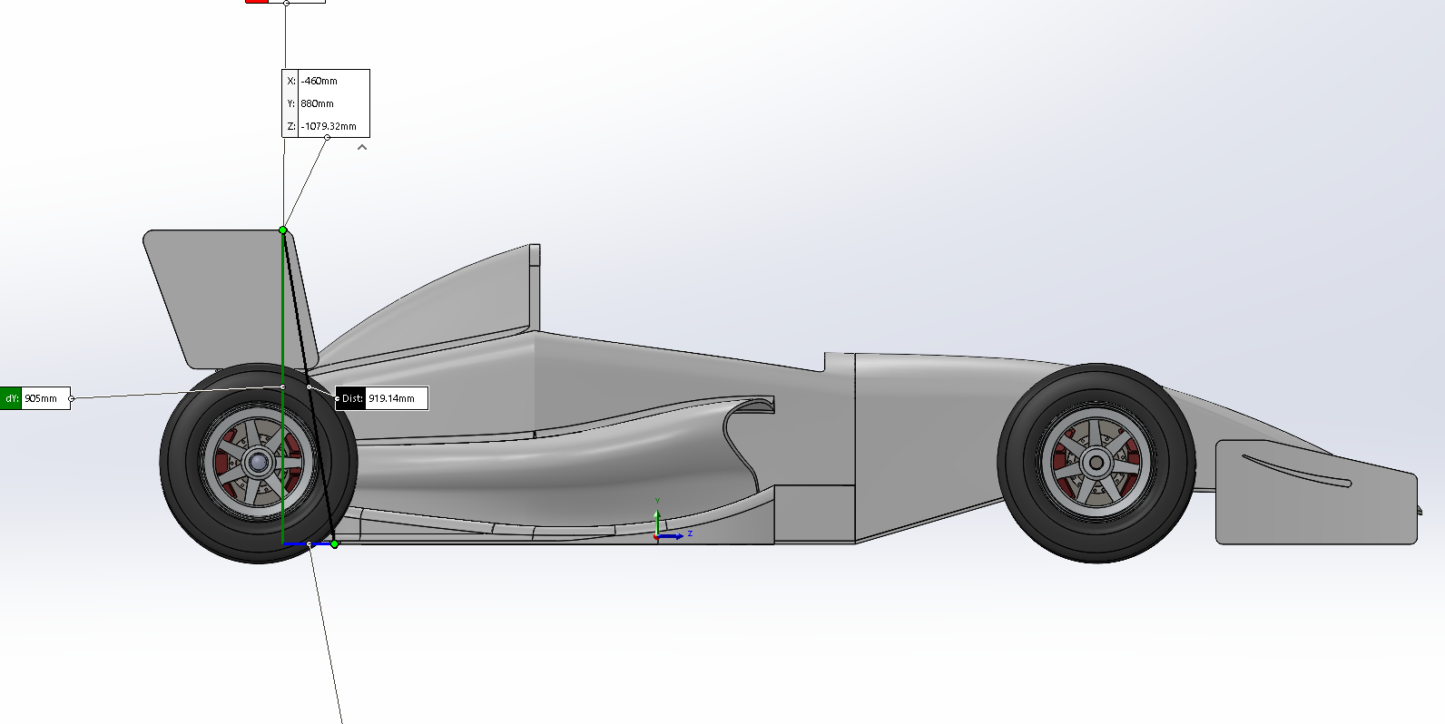
These CAD (computer-aided design) views show the digital model from above and from the side. They help us check dimensions and plan the space around the car for the airflow calculation.
 View full size ↗
 View full size ↗
 View full size ↗
How to read the CAD labels
mm means millimetres; 1,000 mm equals one metre. X, Y and Z name the model’s three coordinate directions. Dist is the straight-line distance between selected points. dY and dZ are changes in position along those directions. Arc Length is the distance along a selected curve. These labels show selected measurements, rather than a complete vehicle specification.
To demonstrate these effects, we compared five versions of an open-wheel, single-seat race car. The original car, shown above, retains its front and rear wings. It establishes a reference for the four changes below.
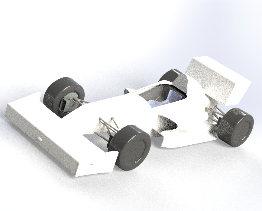
Wings facing the airflow
We turn wing profiles to face more directly into the incoming air. This lets us examine how greater obstruction increases drag.
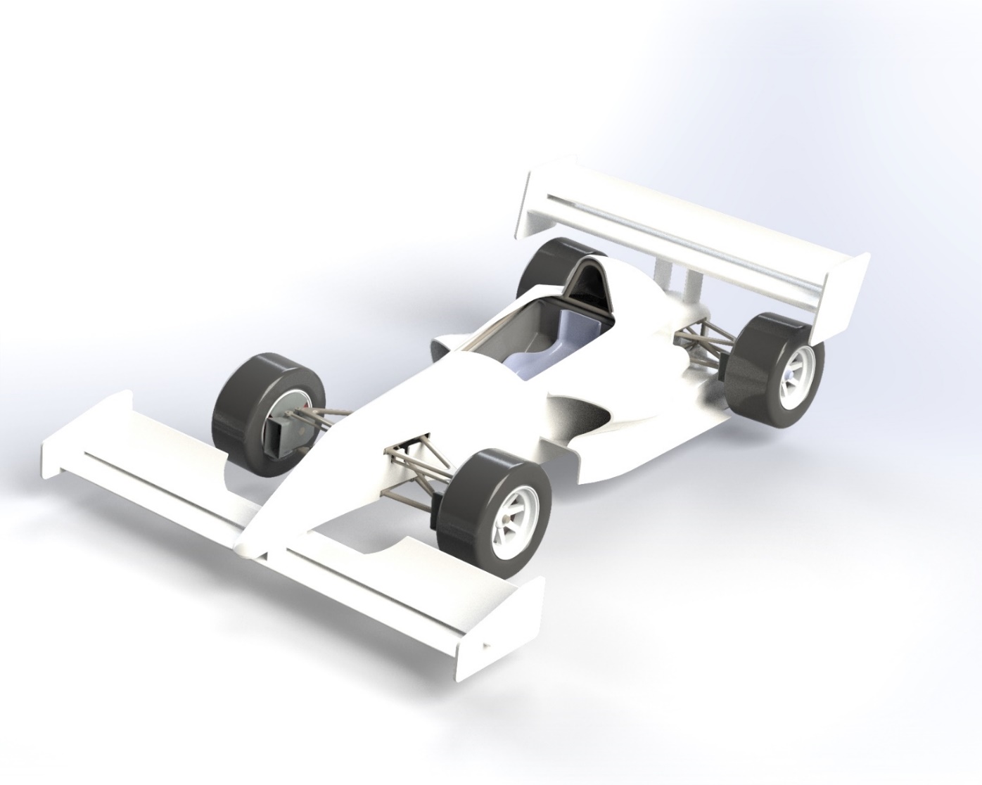
Wider wings
We extend the front and rear wings by 500 mm on each side. This investigates the effect of additional wing area on drag and downforce.
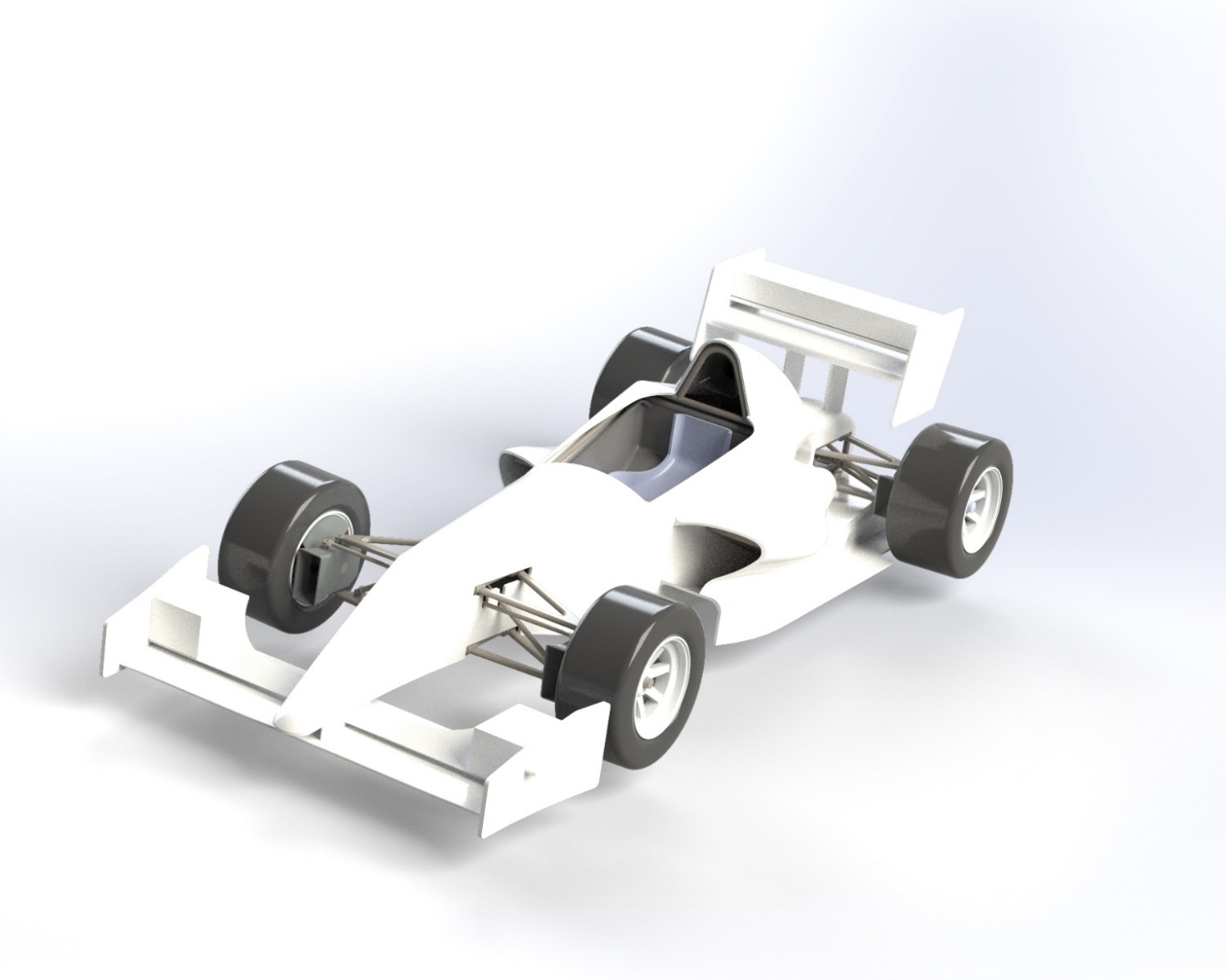
Modified wing elements
We turn small parts of the wing profiles to reduce their downforce contribution. This explores lower aerodynamic loading while keeping frontal area almost unchanged.
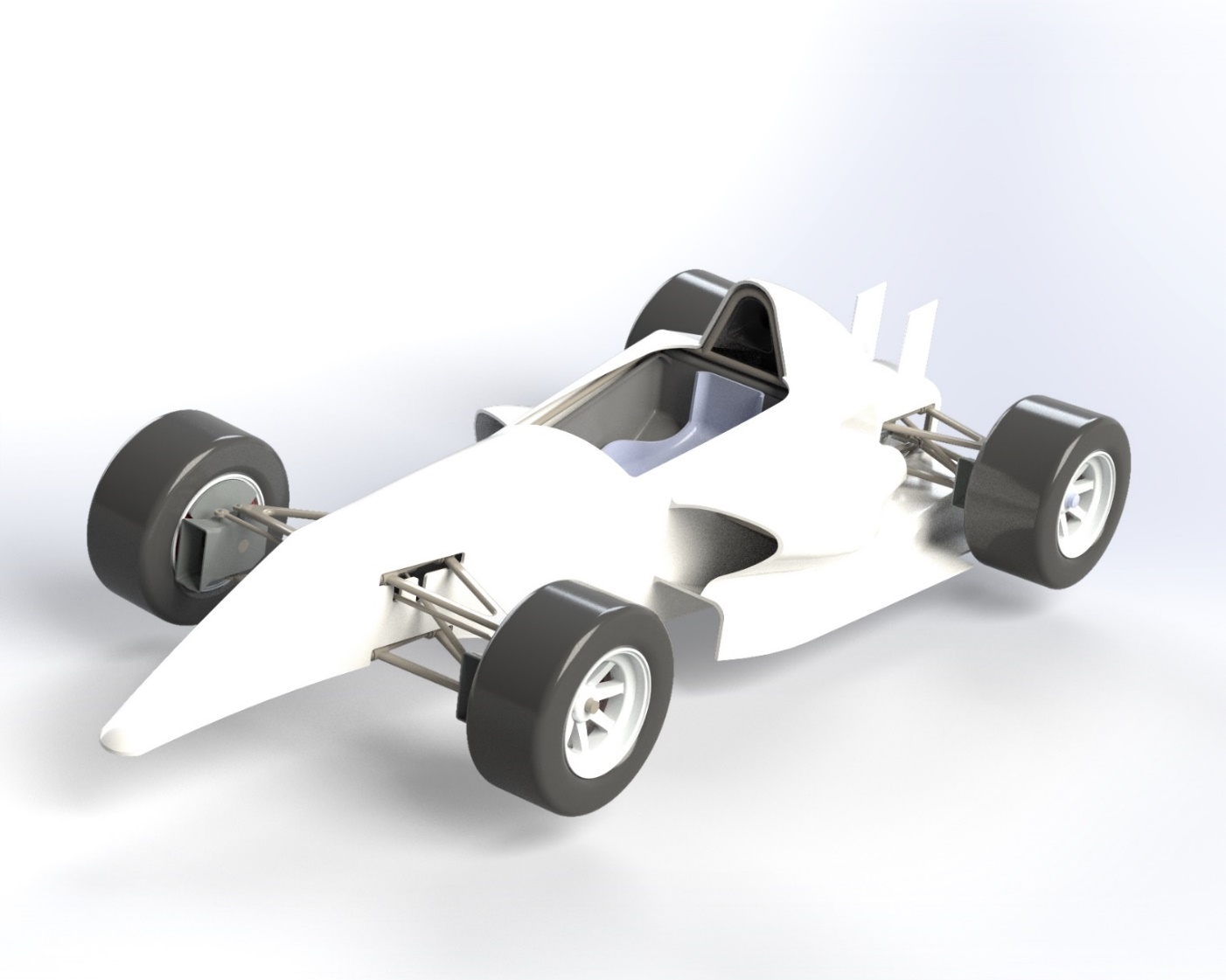
Wings removed
We remove the front and rear wing sections. This identifies the combined contribution of the wings to drag and downforce.
These are deliberately large changes that make their effects easier to compare. They are investigation tools, rather than proposed race specifications.
What does CFD tell us?
CFD divides the space around the car into many small cells, called a mesh. The software calculates airflow through those cells and the pressure and friction acting on the vehicle.
Adding the surface forces gives two important results:
- Drag: the aerodynamic force that opposes forward motion.
- Lift or downforce: the aerodynamic force that lifts the car away from the road or presses it towards it.
Air density is the mass of air in a given volume. We also use coefficients to compare designs. A coefficient expresses a result relative to defined conditions and has no units.
- Drag coefficient · Cd
- Describes drag after accounting for air density, speed and a reference area. Here, that area is the frontal area, A: the size of the car’s outline when viewed directly from the front, measured in square metres (m²).
- Lift coefficient · CL
- Describes vertical aerodynamic force. In our convention, a negative value means downforce. A more negative value means more downforce when the other conditions remain equal.
- Pressure coefficient · Cp
- Describes pressure at a particular location relative to the surrounding airflow. A pressure map helps us understand how different surfaces produce the overall forces. It is the distribution across the car that matters.
For drag comparisons, we use Cd × A, known as drag area. This accounts for both shape and size. Comparing Cd alone can be misleading when a modification also changes frontal area. The small letters d, L and p identify drag, lift and pressure; they are labels, not extra values to multiply.
Seeing where pressure changes
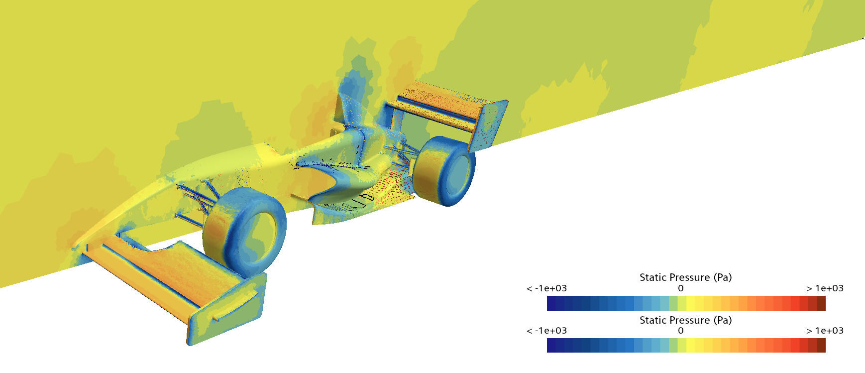
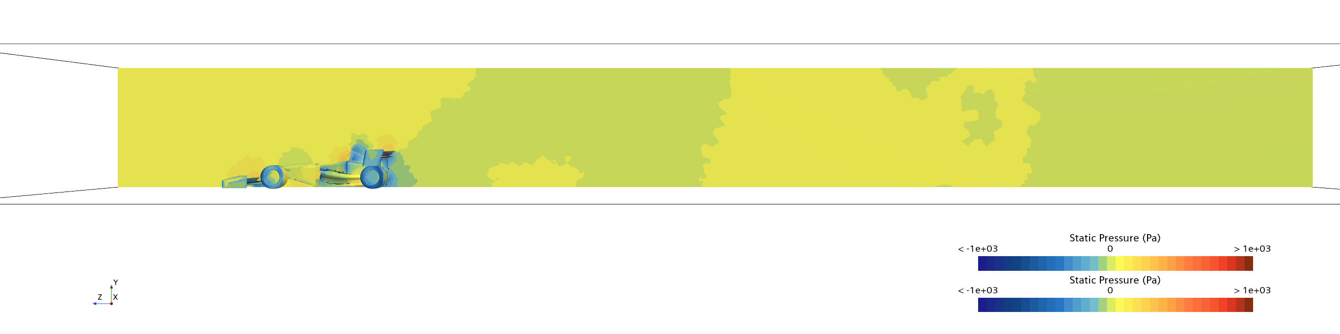
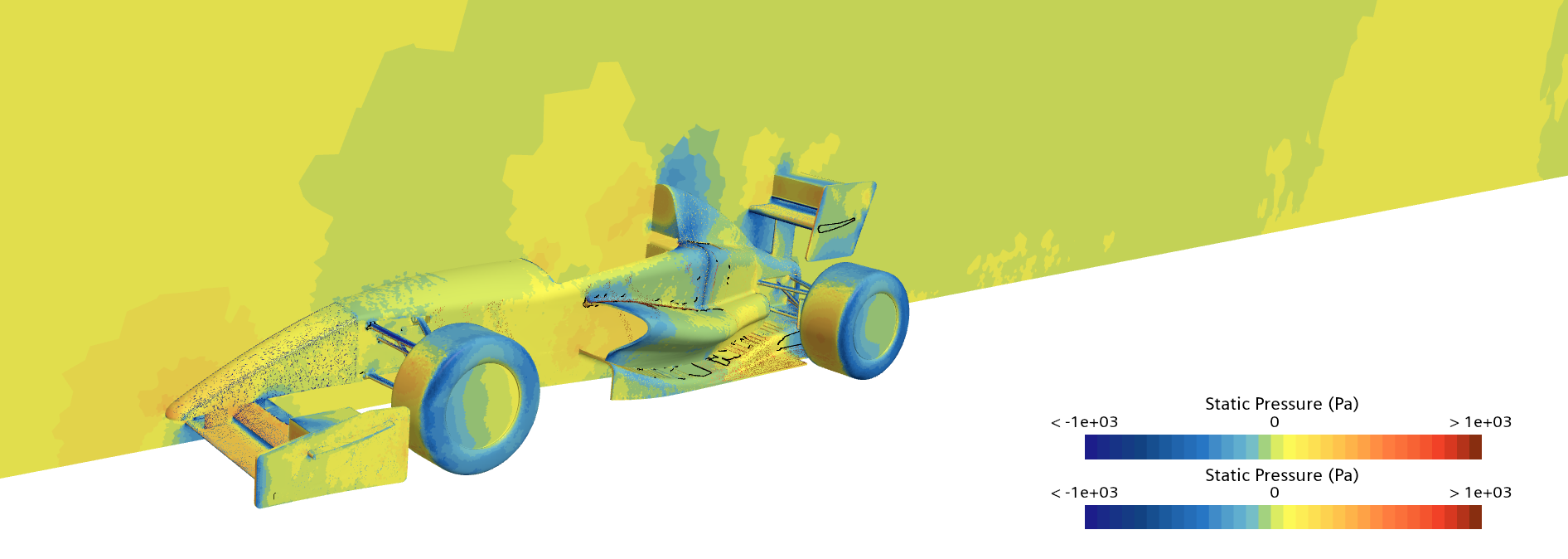
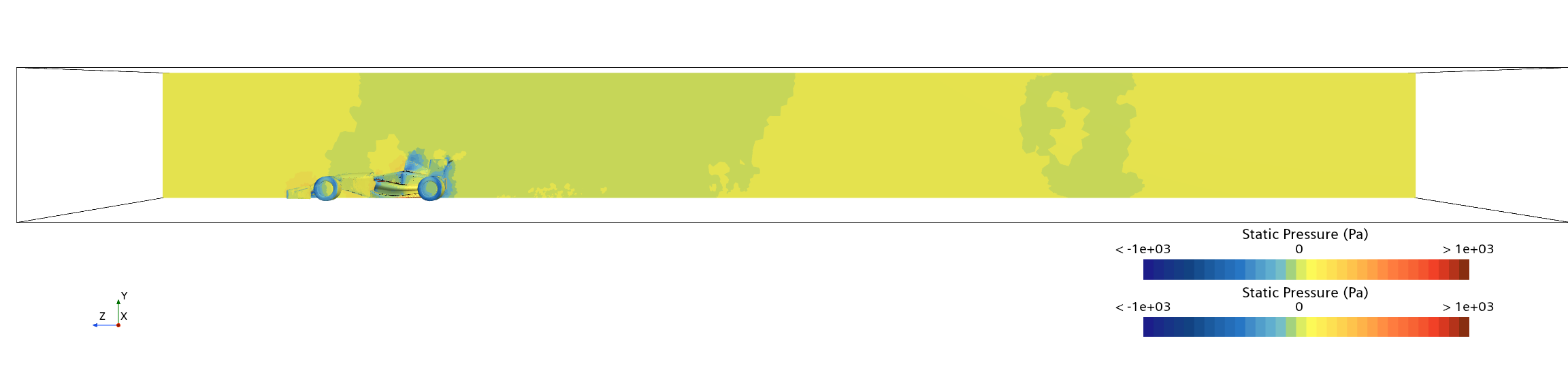
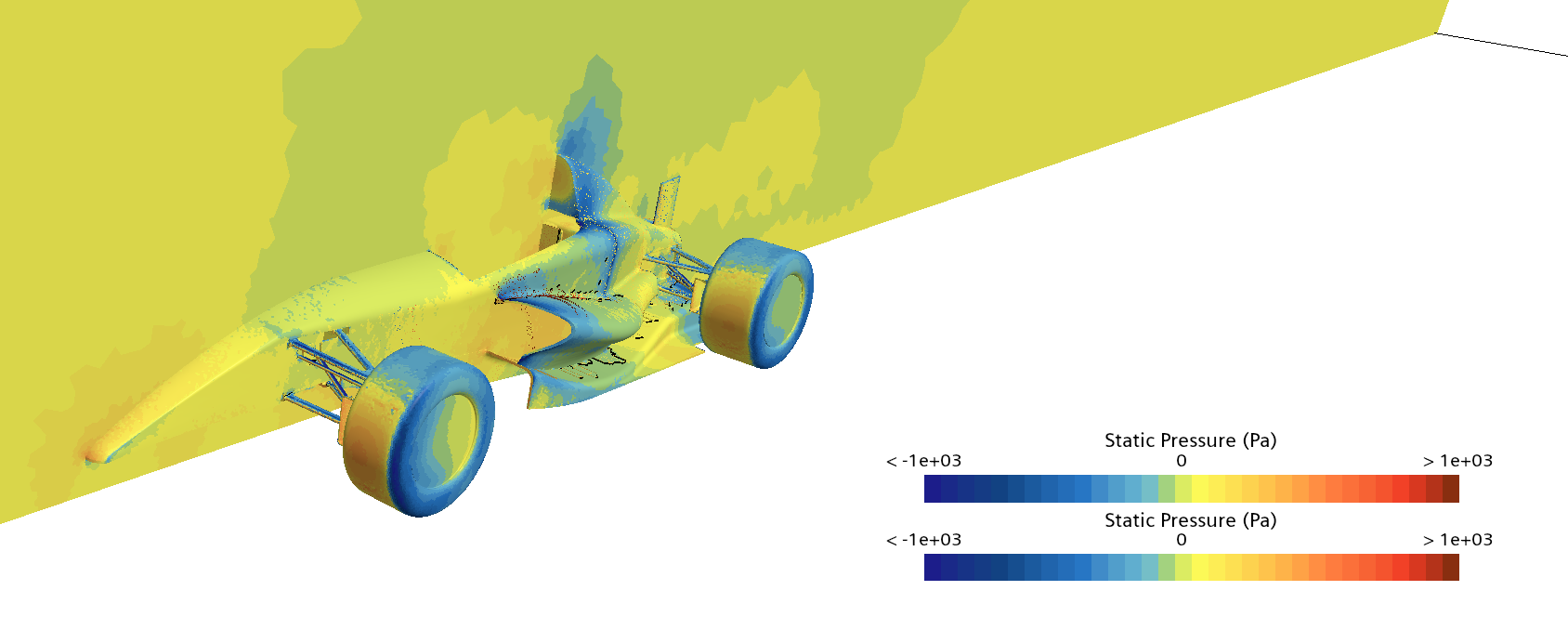
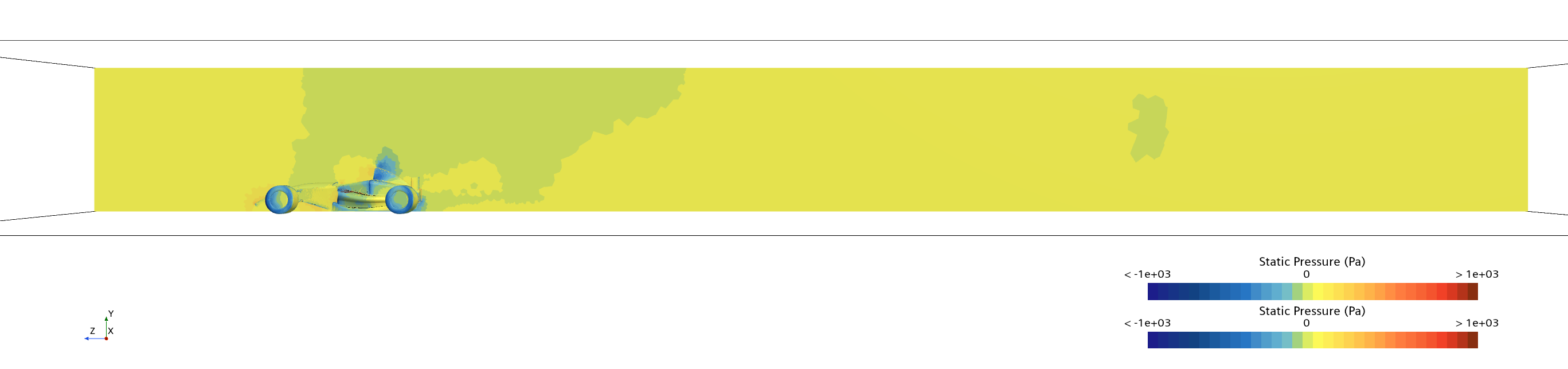
These scenes show static pressure, the local air pressure relative to the simulation’s reference pressure. The coloured slice shows pressure around the car, while the coloured surfaces show pressure acting on its body and wings.
Pa means pascals, a unit of pressure. Blue indicates lower pressure and red indicates higher pressure on the displayed scale. 1e+03 means 1,000; the < and > symbols mark values below or above the scale limits. The two bars, where shown, label the surface and slice displays.
Select a configuration to see its close view and full side view. Open any image to read it at full size.
Original carStatic pressure
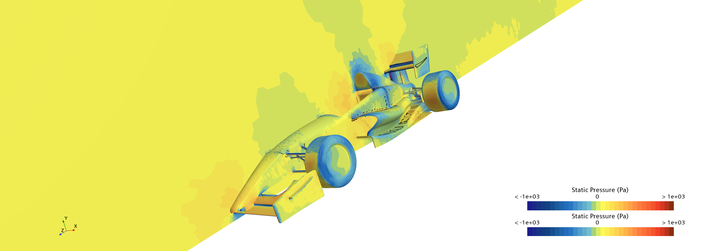 View full size ↗
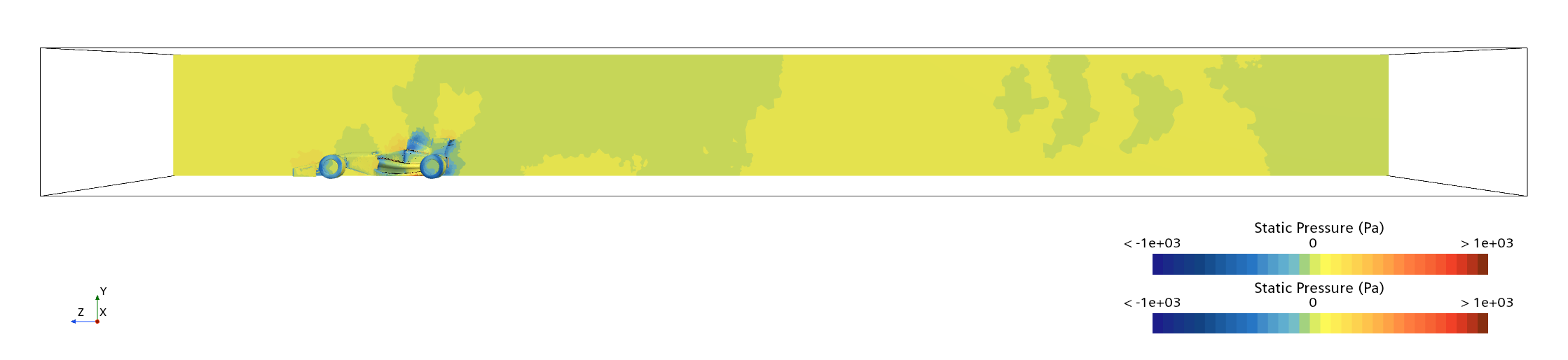 View full size ↗
Wings facing the airflowStatic pressure
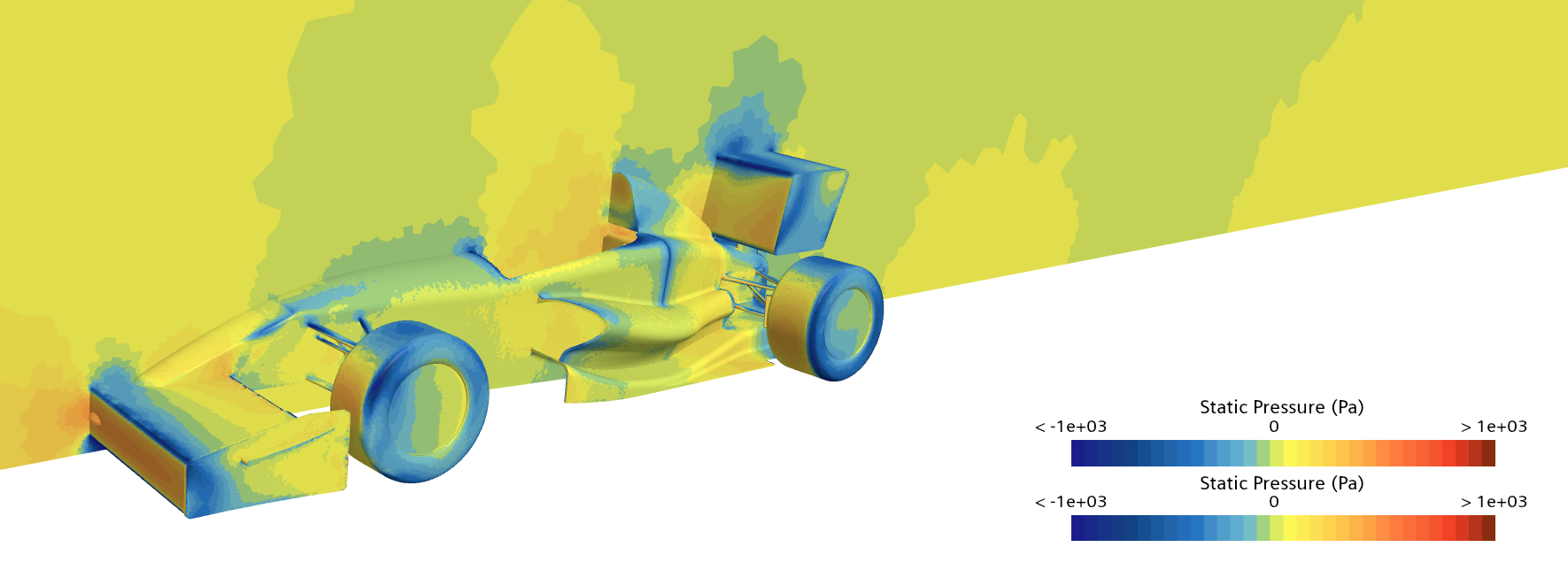 View full size ↗
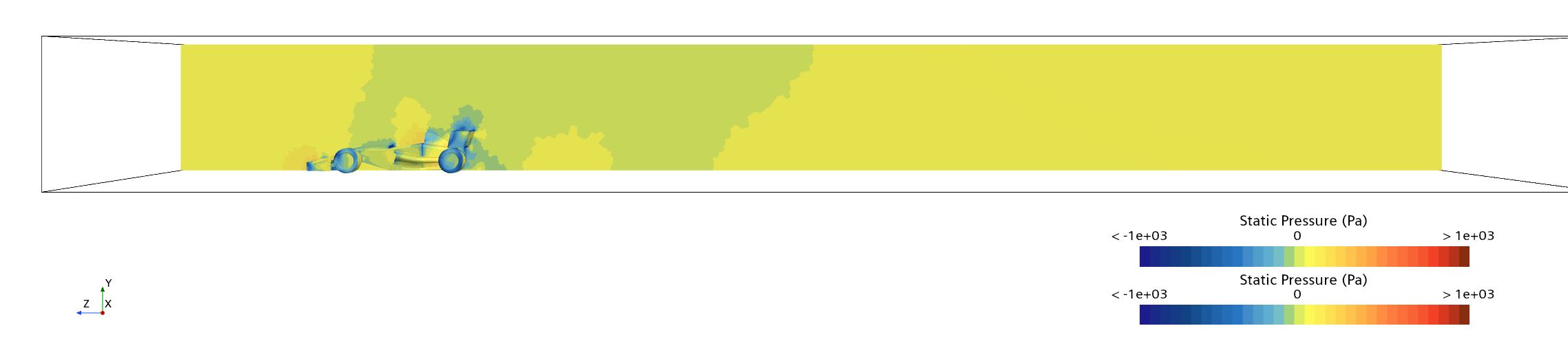 View full size ↗
Wider wingsStatic pressure
 View full size ↗
 View full size ↗
Modified wing elementsStatic pressure
 View full size ↗
 View full size ↗
Wings removedStatic pressure
 View full size ↗
 View full size ↗
These are simulation outputs. The images help explain the airflow; vehicle forces come from adding pressure and friction over the surfaces. Camera framing varies between configurations.
One geometry change can affect several results
The simulations showed that the changes were connected. Extending the wings increased frontal area, but it also increased drag coefficient. Turning the wings towards the airflow changed both drag and downforce.
Compared with the original car, the predicted drag area changed by approximately:
| Configuration | Change in drag area |
|---|---|
| Wings facing the airflow | 37% increase |
| Wider wings | 104% increase |
| Modified wing elements | 6% decrease |
| Wings removed | 36% decrease |
At the same speed and air density, these percentages also describe the predicted change in drag force.
This is why we examine the complete car. A wing operates in airflow affected by the body and wheels, and it changes the air reaching components behind it. Its performance in isolation does not fully describe its effect when fitted.
Maximum speed
A car reaches its power-limited maximum speed when the power available at the wheels equals the power needed to overcome resistance. There is then no spare power to increase speed.
Reducing drag area can raise that limit without increasing engine output. Increasing drag area uses more power at any given speed and can lower the limit.
Our wider-wing configuration therefore introduces a substantial straight-line cost. Removing the wings reduces that cost, but also removes much of their downforce.
Tyre rolling resistance also matters. This comes mainly from the tyres deforming as they roll. Downforce increases the load on the tyres and can increase this resistance.
Gearing provides another limit. A car may reach its maximum permitted engine speed before it reaches the speed that its power and aerodynamic drag would otherwise allow.
Acceleration times
Acceleration depends on the forward force at the tyres after drag and rolling resistance have been subtracted. Dividing that remaining force by vehicle mass gives acceleration.
Near the start of a 0–100 km/h run, aerodynamic forces are relatively small. Tyre grip, engine torque and gearing can have a larger influence. Torque is the engine’s twisting effort; the gears transmit it to the wheels. As speed rises, drag uses more of the available driving force.
We use the CFD results to calculate resistance at successive speeds. A vehicle model then estimates how long the car takes to pass through each speed interval, including any gear changes.
A useful prediction must account for tyre grip, shift time and the energy needed to accelerate rotating parts. It must also consider how acceleration transfers load between the axles.
Downforce can help when tyre grip limits acceleration. Once the car can transmit all its available engine force to the road, extra downforce does not directly provide more forward force. Any associated drag still opposes acceleration.
Seeing how the airflow changes
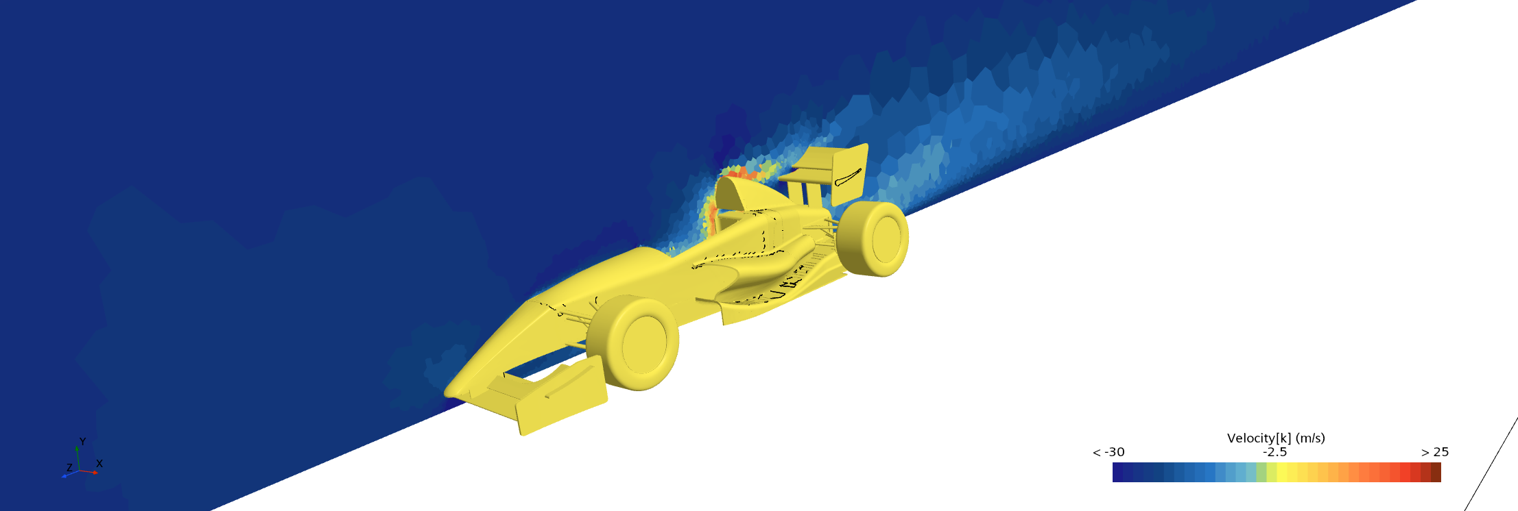
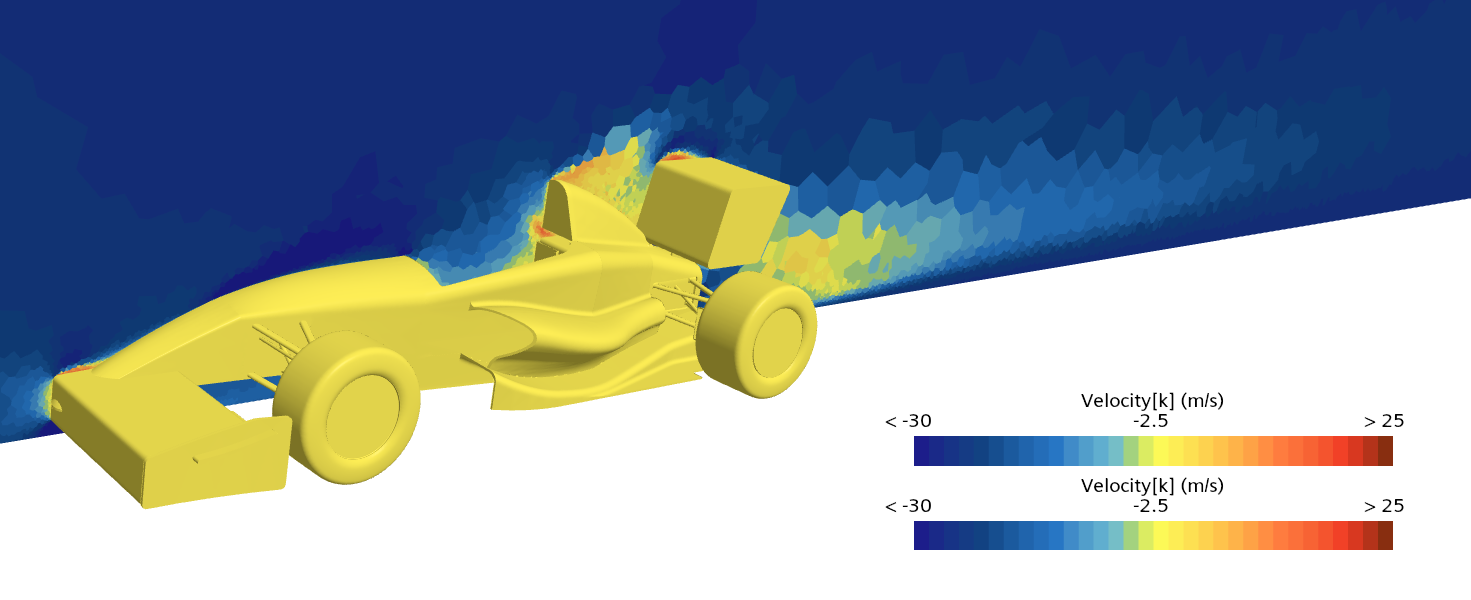
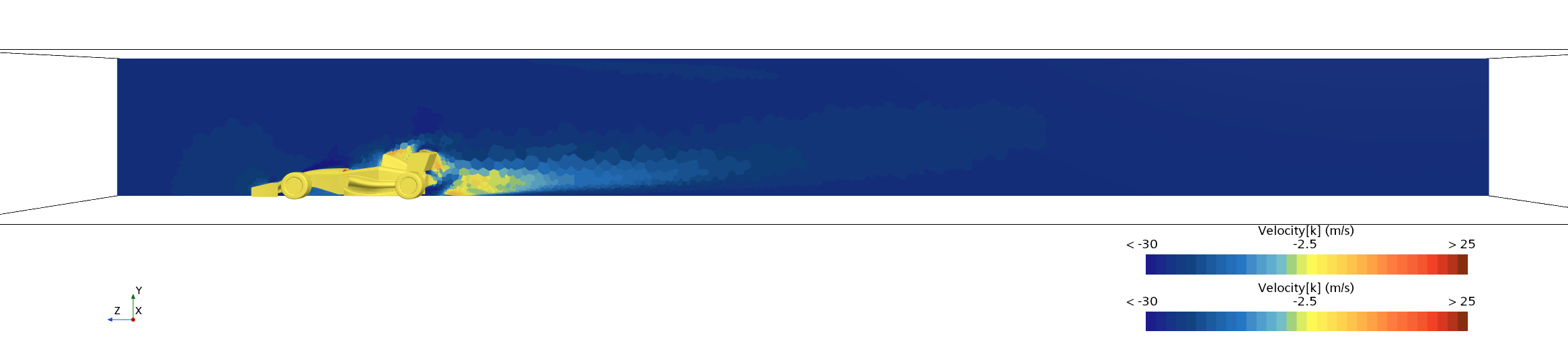
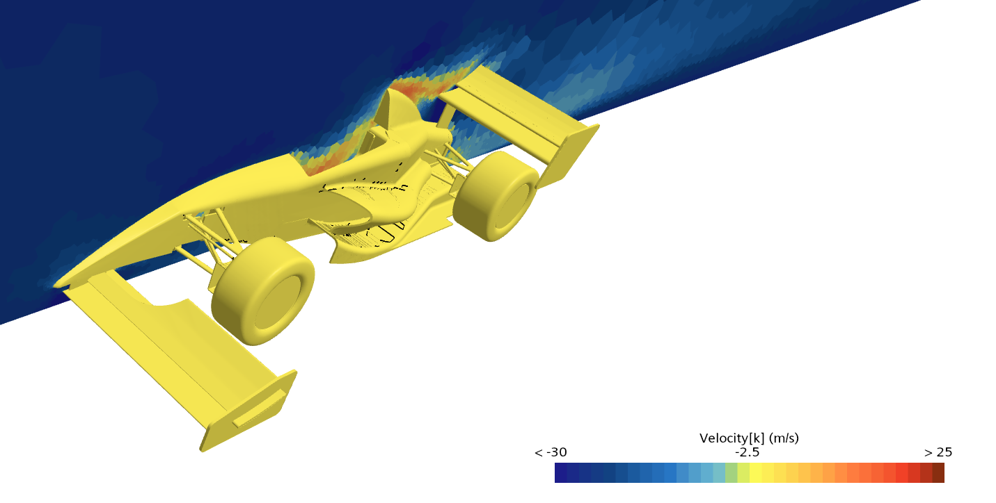
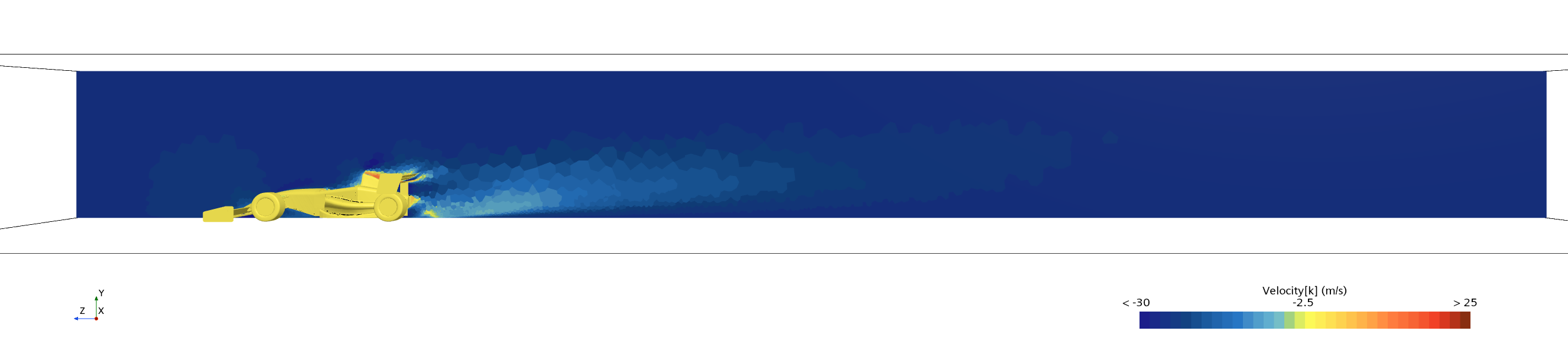
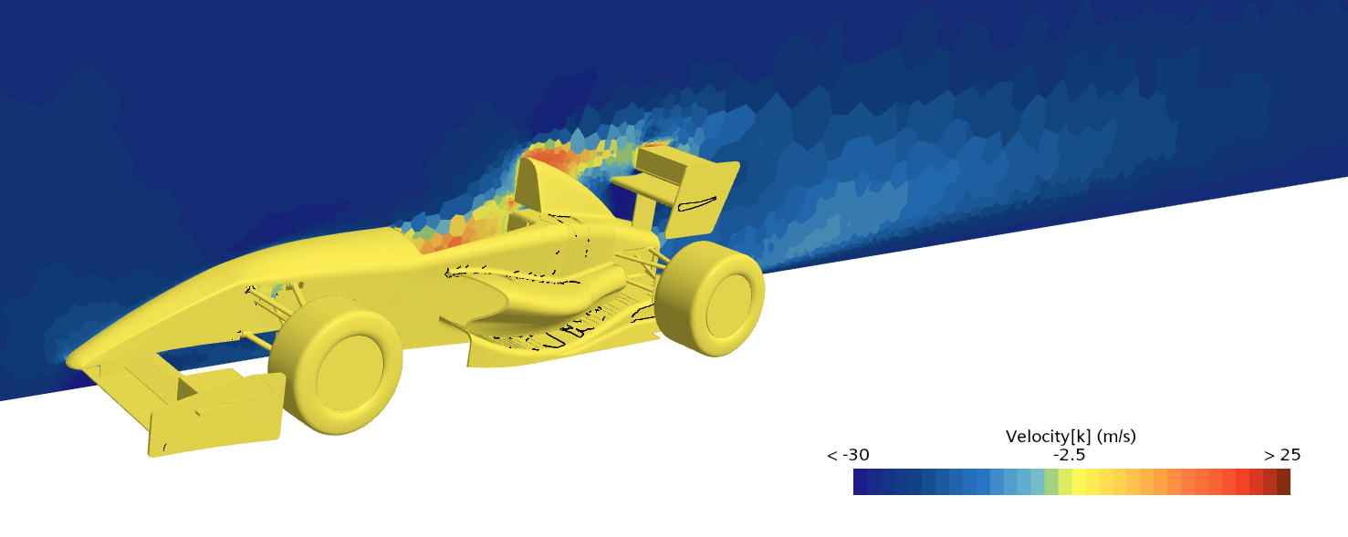
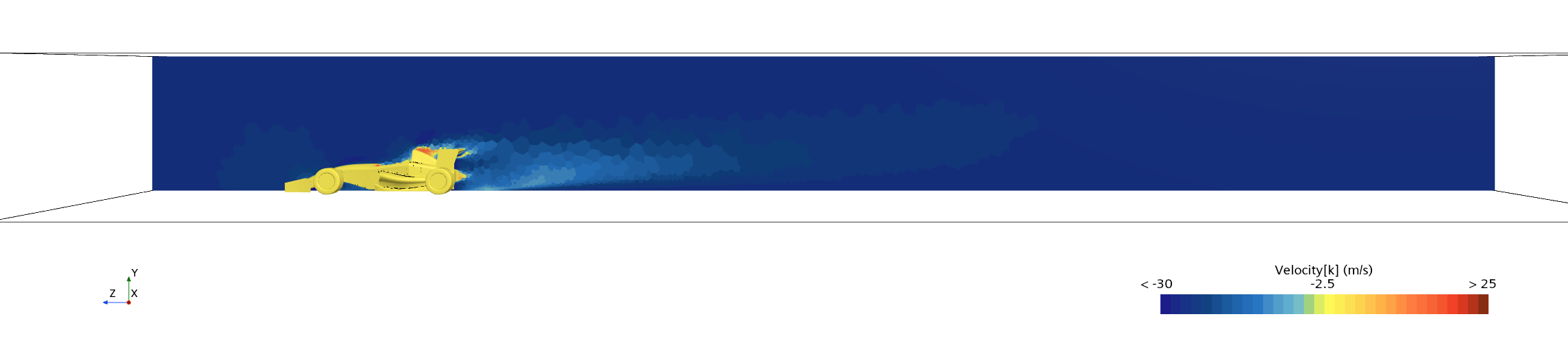
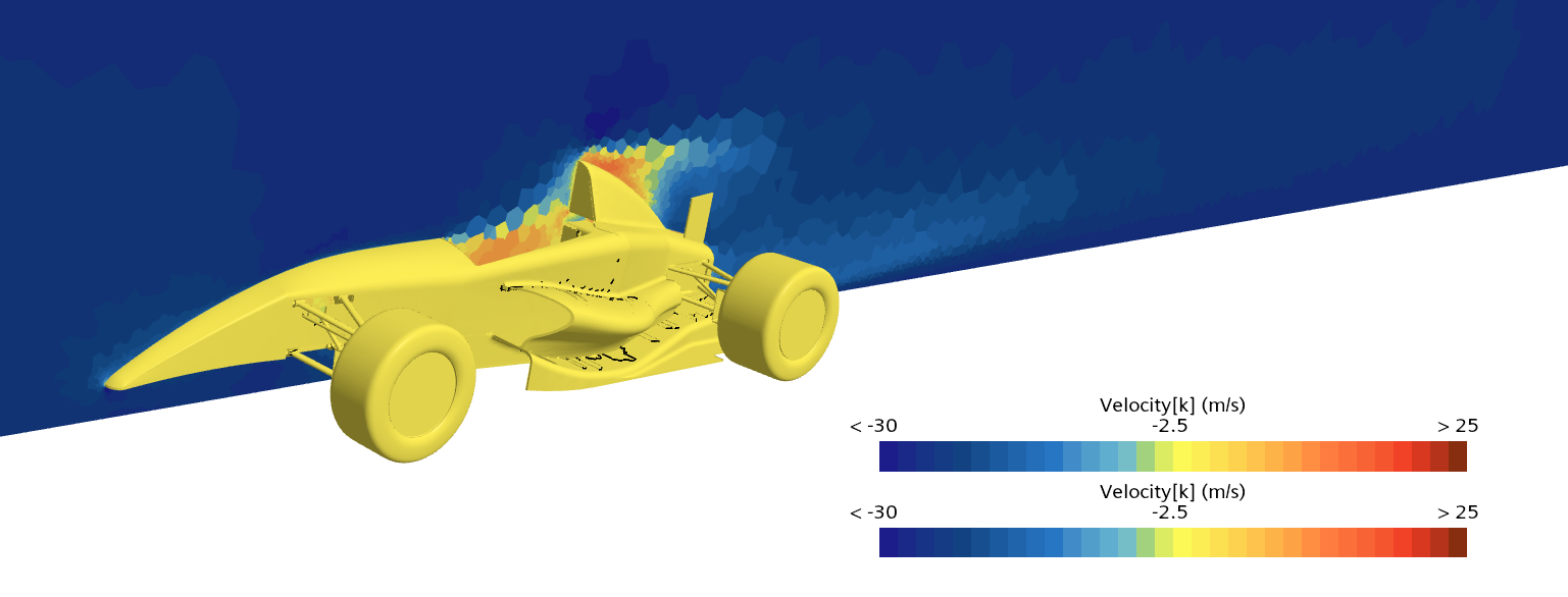
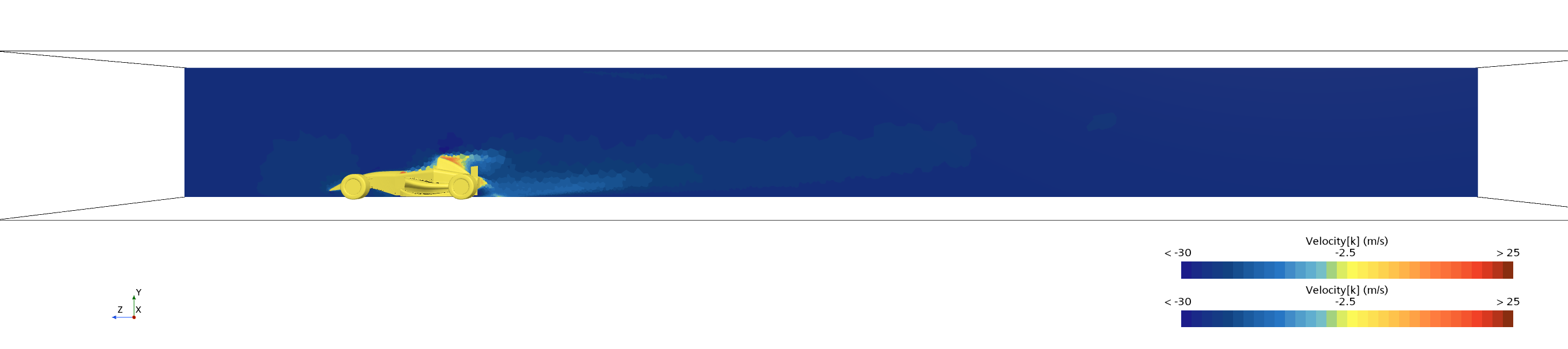
These scenes show the Z-direction component of velocity, labelled Velocity[k]. Here, k identifies the Z direction and m/s means metres per second. A negative value indicates flow towards negative Z: −30 m/s means 30 metres per second in that direction.
The colour therefore describes both the direction and size of this component, rather than total airspeed. The air next to the stationary car surfaces has zero velocity in this simulation. The full side views also show the wake: the region of altered airflow behind the car.
Select a configuration to see its close view and full side view. Open any image to read it at full size.
Original carZ-direction velocity
 View full size ↗
 View full size ↗
Wings facing the airflowZ-direction velocity
 View full size ↗
 View full size ↗
Wider wingsZ-direction velocity
 View full size ↗
 View full size ↗
Modified wing elementsZ-direction velocity
 View full size ↗
 View full size ↗
Wings removedZ-direction velocity
 View full size ↗
 View full size ↗
These are simulation outputs. The images help explain the airflow; vehicle forces come from adding pressure and friction over the surfaces. Camera framing varies between configurations.
Power absorbed by aerodynamic drag
Power absorbed by drag is the rate at which energy is used to overcome air resistance. It equals drag force multiplied by vehicle speed.
With constant air density and unchanged aerodynamic coefficients, drag increases with the square of speed. The power needed to overcome it increases with the cube of speed.
Consequently, doubling speed produces:
- Four times the drag force.
- Eight times the power demand from aerodynamic drag.

For example, overcoming drag at 200 km/h requires eight times the power needed at 100 km/h under these assumptions. This refers to aerodynamic drag alone, rather than total vehicle power demand.
At a fixed speed, drag power is proportional to drag area. Our wider-wing configuration therefore needs approximately twice the original car’s power to overcome aerodynamic drag.
This helps us judge whether the downforce gained from a geometry change justifies its power cost.
Elasticity time: response while already moving
Elasticity time measures how long a car takes to accelerate between two speeds, usually in a specified gear. An 80–120 km/h comparison shows how the vehicle responds while already moving.
We can calculate this in small speed steps, updating driving force and resistance throughout the interval. The gear or shift strategy must remain consistent between designs because it directly affects the force available at the tyres.
Higher drag leaves less force for acceleration and can lengthen the interval. Lower drag can shorten it. Downforce may help where grip is limited, while its associated drag and rolling resistance work against that benefit.
This measure complements a standing-start test because it focuses on performance within an existing speed range.
Using the results to choose a design
For these comparisons, we assume level ground, still air and the same vehicle mass and drivetrain. We also treat each configuration’s aerodynamic coefficients as constant across the speed range.
Real vehicles introduce further changes. Suspension movement alters ground clearance and body angle. Wind changes the airflow direction. Tyres respond differently as their load and temperature change.
CFD lets us investigate these conditions before committing to physical parts. We check the mesh and whether the calculated forces have settled, then use the aerodynamic results in the vehicle performance model. Physical testing can check those predictions.
The design choice depends on the intended use. A car with long straights may benefit from lower drag. A car that spends more time braking and cornering may gain more from additional downforce.
By connecting geometry, airflow and vehicle performance, we can explain what a change provides, what it costs, and why it belongs on the car.
Model credit and special thanks
Special thanks to Dan Serban for creating the CAD model used in this study. His Formula-type single seater provides the starting geometry for the comparisons shown in this article.
Serban, D. (2022) Formula-type single seater. GrabCAD Community [CAD File]. Available at: https://grabcad.com/library/formula-type-single-seater-1/details?folder_id=12079124 (Accessed: 21/10/2025).