
A race car can only use its power, braking force and aerodynamic load through the tyres. To predict how the car will respond, a simulation needs a useful description of what happens at the contact patch. That description is the tyre model.
Our aerodynamics articles examined the forces produced by airflow. This first vehicle dynamics article follows those loads to the road. We compare models fitted to test data, models based on tyre mechanics, and models that learn from data. A cornering example shows why the choice matters.
What must a tyre model describe?
The contact patch is the area where the tyre touches the road. As the tyre rolls, the tread and supporting structure deform. Part of the patch can grip while another part slides. The resulting forces depend on load, slip, camber, pressure, temperature and the road surface.
A model turns selected inputs into forces and moments. The detail required depends on the question. Predicting a steady cornering balance requires different information from studying a rapid steering input or a tyre striking a kerb.
- Vertical load, Fz
- The force that presses the tyre against the road. Vehicle weight, load transfer and aerodynamic load all affect it.
- Slip angle, α
- The angle between the wheel’s heading and its direction of travel. A tyre can generate cornering force at a small slip angle without the whole contact patch sliding.
- Longitudinal slip, κ
- The relative difference between the tyre’s rolling speed and its forward speed. It is relevant during braking and acceleration; the exact definition and sign convention must be stated.
- Cornering stiffness, Kyα
- The initial slope of lateral force against slip angle. Near zero slip, Fy ≈ Kyαα, provided the angle units match. This is not the tyre’s vertical spring stiffness.
Combined slip occurs when a tyre must produce longitudinal and lateral force together, such as during braking into a corner. The two demands interact. Adding the separate maximum braking and cornering forces would overstate the available grip.
What the cornering data shows
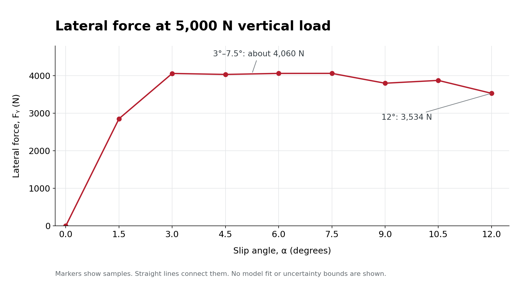
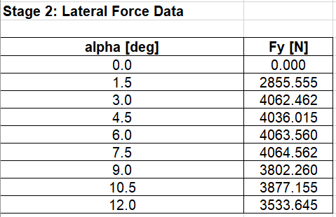
The opening graph uses lateral-force data at 5,000 N vertical load. At 1.5° slip angle, lateral force is about 2,856 N. By 3°, it reaches about 4,062 N. It then remains close to 4,060 N through 7.5°, before falling overall at larger angles.
At 12°, the force is 3,534 N, about 13.1% below the largest sampled value. More slip angle has not produced more useful cornering force. A linear model extended through this range would miss both the broad peak and the reduction beyond it.
| Slip angle | Lateral force | What it shows |
|---|---|---|
| 1.5° | 2,856 N | Force builds rapidly. |
| 3.0° | 4,062 N | The curve is near its broad peak. |
| 7.5° | 4,065 N | The largest value in these samples. |
| 12.0° | 3,534 N | Less lateral force at greater slip. |
The samples do not locate an exact optimum slip angle. The small differences across the broad peak cannot be judged without repeat tests and uncertainty estimates. These values also describe one load condition, not every tyre or every corner.
The second dataset shows how cornering stiffness changes with vertical load. At 4,000 N, it is about 1,864 N/degree. At 8,000 N, it is about 2,405 N/degree. Doubling the load increases the initial cornering response by only 29.0%.
 View full size ↗
This distinction matters when assessing downforce or load transfer. A model must describe how tyre response changes with wheel load. The stiffness curve alone cannot quantify the resulting gain in maximum cornering force.
Inspect the complete numerical datasets
 View full size ↗
 View full size ↗
Magic Formula: fit the measured response
An empirical model describes measured behaviour with a fitted equation. The Magic Formula, associated with Pacejka, is a familiar example. Its coefficients control the force curve’s shape, slope, scale and curvature. They do not directly describe the rubber compound or tyre construction.
This makes it useful for a vehicle simulation. Once calibrated, a compact equation can reproduce a nonlinear force curve quickly. Extended versions add relationships for load, camber, combined slip and other effects, which is why the wider model family is also described as semi-empirical.
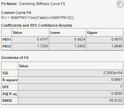
For the stiffness curve above, a two-coefficient fit uses a reference load of 5,000 N, with PKY1 ≈ 0.4747 and PKY2 ≈ 1.7200 in this unit convention. It predicts about 2,063 N/degree at 5,000 N, compared with the data value of 2,036 N/degree.
See the stiffness-fit coefficients and statistics
 View full size ↗
A close fit is useful, but it does not prove accuracy outside the tested conditions. A curve calibrated at one temperature or pressure needs further evidence before it describes a different condition. Large slip is not automatically beyond Magic Formula’s scope; the relevant limit is the range and quality of its calibration.
A basic steady-state curve also has no memory of how a force developed. Pacejka and Besselink’s transient formulation shows that the model family can include force build-up and combined slip. These features must be present and calibrated in the implementation used.
TMeasy: a compact handling model
TMeasy combines simplified physical ideas with measured tyre characteristics. Parameters describe features such as the initial slope, peak force and sliding behaviour. It uses longitudinal and lateral characteristics to construct a combined-slip response.
The relatively compact parameter set can make setup easier when detailed tyre data are limited. This suits early handling studies and repeated vehicle simulations. Parameters can be estimated initially, then improved with measurements. An estimate remains an estimate, however, until it is checked against the tyre of interest.
Rill’s published TMeasy formulations include contact calculations and transient behaviour. It is therefore too broad to describe TMeasy as unable to model contact or slip. Its reduced description does not, by itself, resolve tread stress, heat generation and wear in the detail needed for tyre construction development.
For a race car, the key check is whether that compact model reproduces the relevant loads and combined braking–cornering conditions. A good fit to separate force curves does not guarantee the same quality when both forces act together.
Physical models: follow the deformation
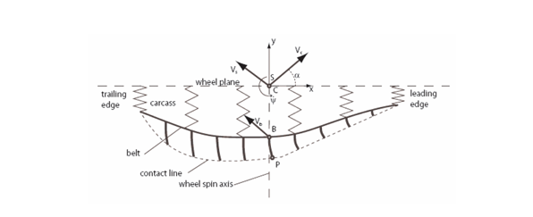
A physical model starts from the mechanisms that create force. A simple brush model represents the tread as flexible elements. They deform while gripping the road and can slide when the local friction limit is reached. Adding their contributions gives the total force.
TreadSim develops this idea by following a tread element through the contact patch and accounting for the supporting tyre structure. Repeating the calculation across the patch produces forces and an aligning moment, the moment that contributes to steering response.
 View full size ↗
The inputs include slip angle, camber, longitudinal slip, vertical load, forward speed, path curvature and inflation pressure. The calculation links contact forces and carcass deformation, so changes to a structural parameter can affect several outputs at once.
 View full size ↗
This approach helps investigate why behaviour changes, but physical detail does not ensure accuracy. In Uil’s reference-tyre comparison, the tested TreadSim implementation overpredicted peak lateral friction at higher loads and generally underpredicted longitudinal friction. Contact-patch shape and pressure assumptions were identified as areas for improvement.
That result concerns one implementation and dataset. It does not establish that all physical models are unsuitable for racing. Simple brush models can be efficient. Flexible structural and finite element models require more inputs and computing effort, but can answer questions about deformation that a fitted force curve cannot.
Neural networks: learn from data
A neural network learns a relationship between inputs and outputs from examples. With suitable training data, those inputs could include slip, load, pressure and temperature. The output could be a tyre force or a parameter used by another model.
A deep neural network has multiple hidden layers. Greater depth does not automatically improve accuracy, make a model physical, or remove the need for measurements. Results depend on the architecture, training data and tests on cases withheld from training.
There are also useful applications short of replacing the entire tyre model. Gräber and colleagues (2021) combined a vehicle model with a neural network that estimated tyre stiffness and friction parameters. Salari and colleagues (2023) investigated tyre normal-force estimation. These are specific estimation tasks, not proof that neural networks outperform every force model.
Training and collecting representative data can be expensive. Running a trained network may be fast enough for real-time use. The main concern is whether it remains reliable when conditions change. An unfamiliar compound, wet surface or temperature range can take it outside its training data.
A combined approach can retain known vehicle physics and use learning for uncertain terms. It still needs independent checks, sensible output limits and a defined range of use.
Which method suits the task?
Model complexity is not a ranking of quality. Choose the outputs, operating range and response speed required, then assess whether the available data can support them. The comparison below is qualitative; the example dataset has not been run through every model listed.
| Method | Useful for | Main benefit | Main limit |
|---|---|---|---|
| Linear stiffness | Small-slip response and initial handling checks. | Fast and easy to interpret. | Cannot represent saturation or the fall beyond peak force. |
| Magic Formula | Handling and lap simulations within a measured range. | Fast evaluation of nonlinear force curves. | Needs suitable data and extensions for the required effects. |
| TMeasy | Compact vehicle handling and setup studies. | A manageable parameter set with combined-slip capability. | Reduced detail; combined response still needs validation. |
| Brush / TreadSim | Contact mechanics and sensitivity to physical assumptions. | Links forces to tread and structural deformation. | Friction and contact assumptions can dominate the error. |
| Detailed structural / finite element | Tyre construction, local stresses and detailed contact. | Resolves more of the tyre structure. | More material data, setup and computing effort. |
| Neural network / combined model | Learning force relationships or estimating uncertain parameters. | Can capture complex relationships in representative data. | Unseen conditions and physical consistency require checks. |
For a steady cornering or lap study, a calibrated handling model can be sufficient. For turn-in or rapid brake release, force build-up matters too. For tyre construction or local contact stress, a more detailed physical model is appropriate. The model must serve the decision.
Check more than the curve fit
Fitting software adjusts parameters to reduce residuals, the differences between predictions and data. MATLAB and Excel Solver can reach similar results because they minimise a similar sum of squared residuals. Agreement checks the numerical fitting process; it is not independent evidence of tyre accuracy.
The fitting setup matters. Starting values and evaluation limits can determine whether an optimiser reaches a useful solution. A high R² can still hide the wrong small-slip slope or a unit error. For example, 2,063 N/degree is about 118,200 N/radian. A stiffness value must be converted before it is used in an expression that expects radians.
A practical validation sequence is:
- Define the conditions. Record tyre specification, load, pressure, temperature, camber, speed and surface.
- Check the implementation. Confirm angle units, slip signs, initial stiffness, peak force and physically sensible behaviour.
- Fit the required range. Include combined slip and changing conditions when the intended simulation requires them.
- Test independent data. Compare against runs excluded from fitting, and assess errors alongside measurement uncertainty.
- Check the complete vehicle. Compare predicted balance and response with track measurements. Investigate tyre, suspension, aero and input errors together.
The example here provides useful stiffness and pure-cornering data. It does not validate braking, combined slip, heat, wear or transient response. No comparison of model accuracy on those tasks can be calculated from these samples alone.
From a tyre model to a setup decision
The 5,000 N example shows why a constant grip value or an unlimited linear force curve is insufficient near the tyre’s limit. The stiffness data shows why the response must also change with load. Both affect how a simulation represents braking, cornering balance and the use of aerodynamic load.
Empirical models offer efficient force predictions within a calibrated range. Physical models help explain the mechanisms and examine structural changes. Neural networks can add useful estimates when the data supports them. Each approach has a role; none removes the need to compare predictions with measurements.
A useful motorsport tyre model captures the effects that matter for the intended manoeuvre, runs within the available time and has evidence for its operating range. That is what allows a predicted setup improvement to support a decision on track.
Data and further reading
The numerical example uses Oxford Brookes University cornering-stiffness and lateral-force data. The tyre identity and repeatability ranges are not specified. The opening chart is replotted from the lateral-force samples; it contains no fitted force curve. The stiffness graph, fit output and two data tables retain their original content. TreadSim diagrams are credited below and in their captions.
- Pacejka, H. B. (2002). Tyre and Vehicle Dynamics. Butterworth-Heinemann. TreadSim contact diagram.
- Pacejka, H. B. and Besselink, I. J. M. (1997). Magic Formula Tyre Model with Transient Properties. Vehicle System Dynamics, 27(S1), 234–249.
- Rill, G. (2013). TMeasy — The Handling Tire Model for all Driving Situations. Proceedings of DINAME 2013.
- de Hoogh, J. (2005). Implementing inflation pressure and velocity effects into the Magic Formula tyre model. Eindhoven University of Technology. TreadSim inputs and calculation structure.
- Uil, R. T. (2007). Tyre models for steady-state vehicle handling analysis. Eindhoven University of Technology. Thesis dated December 2007; degree awarded in 2008.
- Gräber, T., Schäfer, M., Unterreiner, M. and Schramm, D. (2021). Application of Neural Networks to External Parameter Estimation for Nonlinear Vehicle Models. SAE International Journal of Connected and Automated Vehicles, 4(3), 297–312.
- Salari, A. H., Mirzaeinejad, H. and Mahani, M. F. (2023). Tire normal force estimation using artificial neural networks and fuzzy classifiers: Experimental validation. Applied Soft Computing, 132, 109835.