
A car’s aerodynamic performance changes when air meets it at an angle. In this CFD study, increasing yaw moves the lift coefficient towards zero and eventually into lift. The drag coefficient also changes, but its lowest value does not identify the best condition for the car.
Our first aerodynamics article examined changes to the vehicle’s shape. Here, we keep the original single-seat car and compare five airflow angles. This shows why straight-ahead performance is only one part of an aerodynamic assessment.
What yaw means
Aerodynamic yaw angle describes the horizontal angle between the car’s forward axis and its direction of travel relative to the air. At 0°, the air approaches the car directly from the front. At non-zero yaw, it approaches from one side as well.
A crosswind can create this condition even when the car travels straight. A car that moves partly sideways can also experience yaw. The angle is different from yaw rate, which measures how quickly the car rotates.
We compared the same geometry at 0°, 5°, 15°, 30° and 45°. The larger angles explore behaviour well away from straight-ahead flow. These fixed-angle cases do not reproduce a complete corner, including steering, body roll and changing tyre loads.
The same geometry at five angles
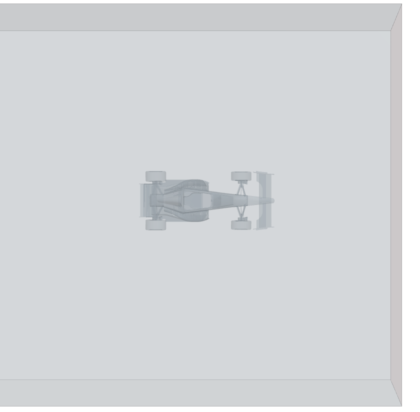
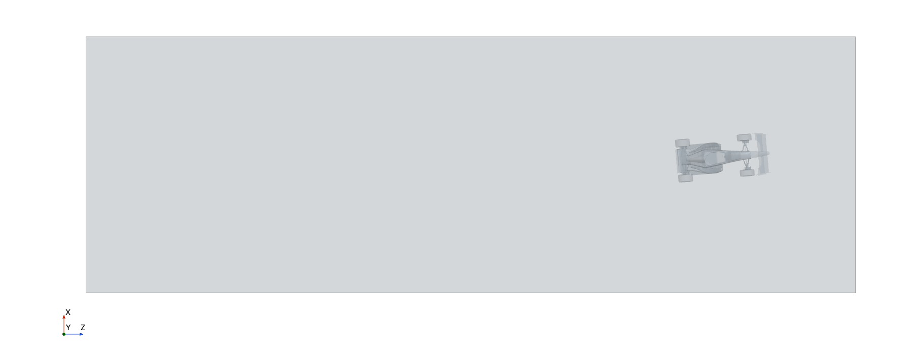
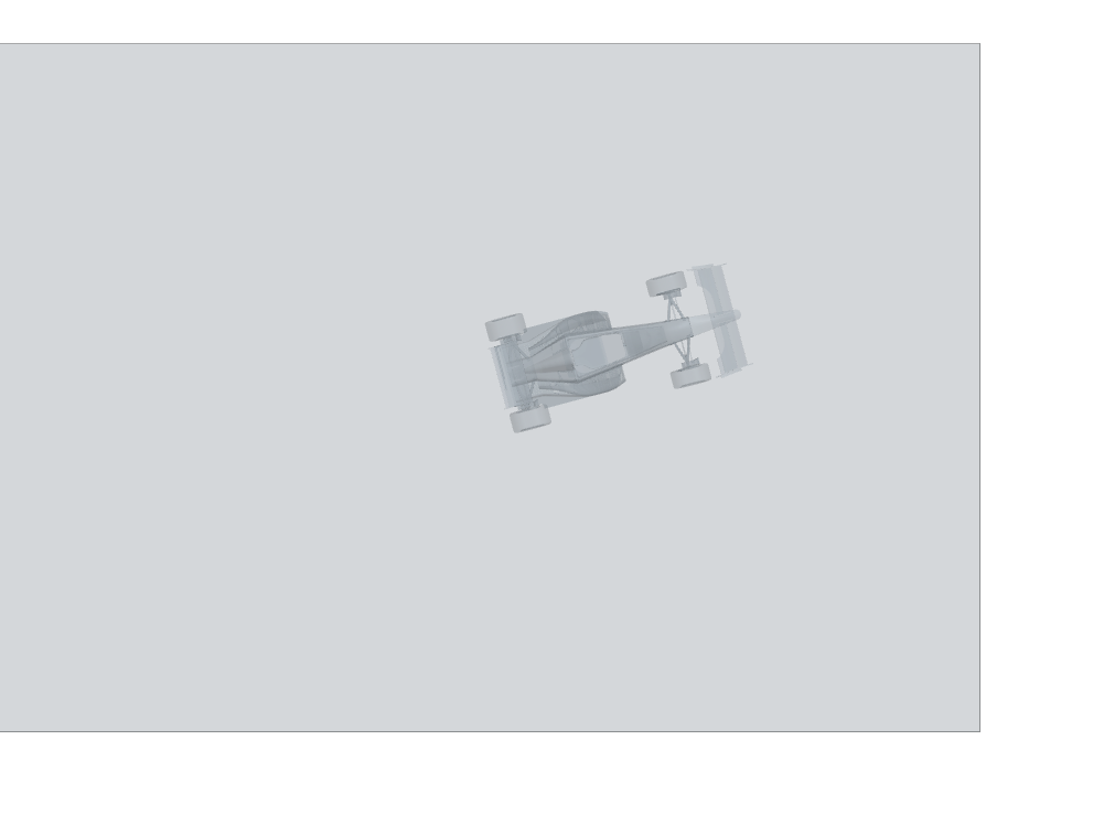
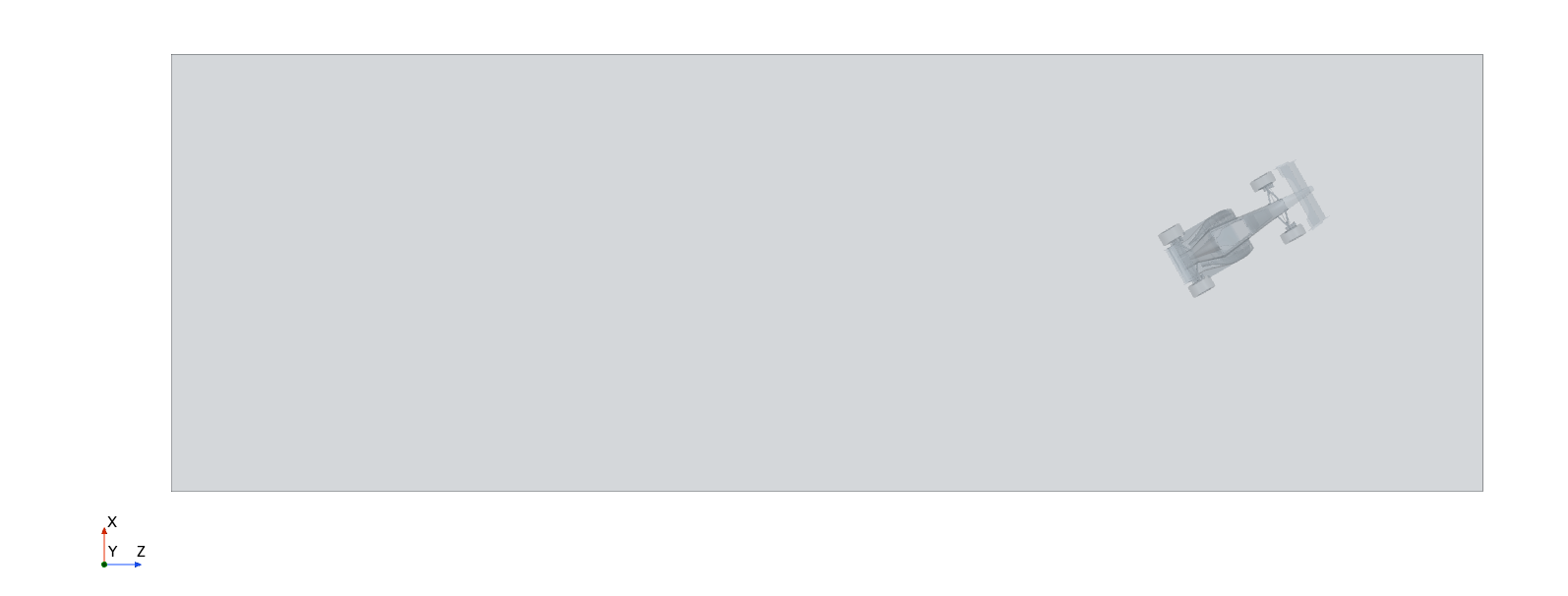
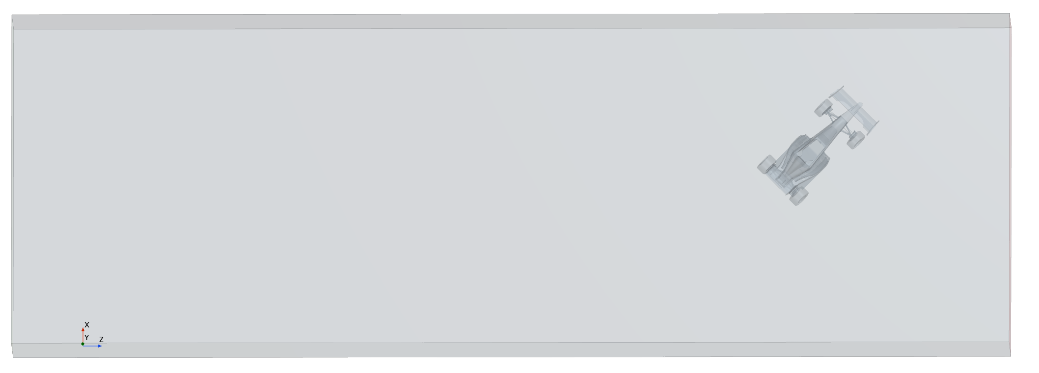
Open an angle to see the model in its surrounding air volume. Camera framing varies; these images are not drawings at a common scale.
0° yawTop geometry view
 View full size ↗
5° yawTop geometry view
 View full size ↗
15° yawTop geometry view
 View full size ↗
30° yawTop geometry view
 View full size ↗
45° yawTop geometry view
 View full size ↗
What changed in the five cases
Projected area, A, is the size of the vehicle’s outline when viewed along the incoming airflow. It increases as more of the car’s side becomes visible. Here, it rises from 1.128 m² at 0° to 2.236 m² at 45°, an increase of about 98%.
Drag coefficient, Cd, describes drag relative to air density, airspeed and a specified reference area. Lift coefficient, CL, describes vertical aerodynamic force. Negative CL means downforce; positive CL means lift.

| Yaw | Area A (m²) | Drag Cd | Pressure output Cp* | Lift CL |
|---|---|---|---|---|
| 0° | 1.1281 | 1.4437 | 1.3724 | −1.9026 |
| 5° | 1.3075 | 0.8883 | 0.8339 | −1.0648 |
| 15° | 1.4659 | 0.6074 | 0.5565 | −0.8056 |
| 30° | 1.8678 | 0.7322 | 0.6883 | −0.5147 |
| 45° | 2.2365 | 0.1230 | 0.0796 | 0.0138 |
*Cp normally describes pressure at a defined location relative to the surrounding flow. The sampling or averaging method for this recorded scalar output is not specified. It is retained here for completeness, but it cannot establish the pressure distribution or total vehicle load.
The largest step in CL occurs between 0° and 5°: its magnitude falls by about 44%. This is a coefficient change, not automatically a 44% loss of downforce, because the area values also change.
By 45°, CL is slightly positive. This calculation therefore predicts lift rather than downforce, although the value is close to zero. Cd follows a different pattern: it falls to 15°, rises at 30°, then falls sharply at 45°. The drag response is not a steady decrease with yaw.
Why drag coefficient is only part of the answer
A larger projected area does not by itself prove that drag increases. Equally, a lower Cd does not by itself prove that drag falls. To calculate force, the coefficient must be paired with the reference area used to define it.
Drag forceD = ½ × ρ × U² × Cd × Aref
Downforce, positive towards the roadFdown = −½ × ρ × U² × CL × Aref
Here, ρ is air density, U is airspeed relative to the car, and Aref is the reference area for the relevant coefficient. At equal air density and airspeed, the products CdAref and −CLAref determine the respective forces.
A worked comparison using the listed areas
The products below assume that each listed projected area was also used to normalise both coefficients for that case. The available results do not confirm those settings. These are conditional calculations, not verified force measurements.
| Yaw | Cd × A (m²) | −CL × A (m²) |
|---|---|---|
| 0° | 1.629 | 2.146 |
| 5° | 1.161 | 1.392 |
| 15° | 0.890 | 1.181 |
| 30° | 1.368 | 0.961 |
| 45° | 0.275 | −0.031 |
Under this assumption, the 5° case has about 29% less drag and 35% less downforce than the 0° case at equal airspeed and density. At 30°, the drag product is higher than at 15°, while the downforce product continues to fall.
The very low Cd at 45° needs particular care. Drag is measured along the relative airflow. A force measured along the car’s forward axis can differ at yaw. The force directions and reference areas must be confirmed before these outputs are used to predict vehicle performance.
What the flow scenes show
Yaw changes how the air reaches the wings, wheels and body. It can change surface pressures and move the disturbed flow behind one component onto another. These are possible explanations for the force changes; the images help us decide where to investigate further.
Pressure around the car
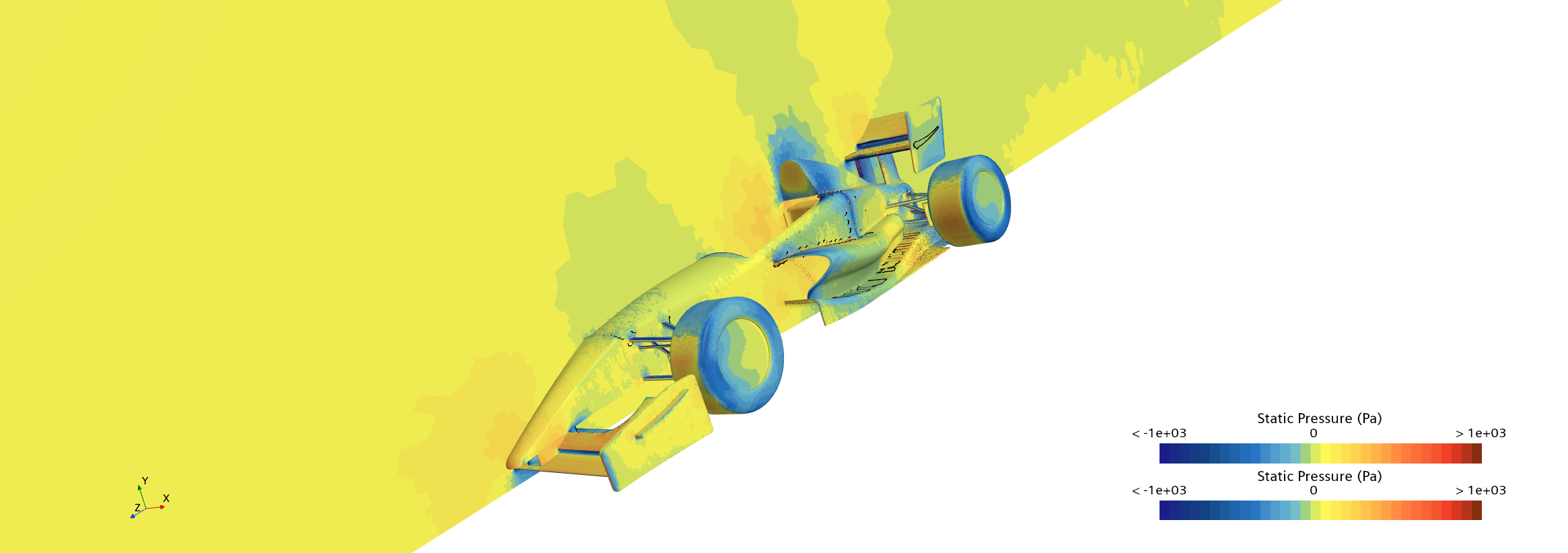
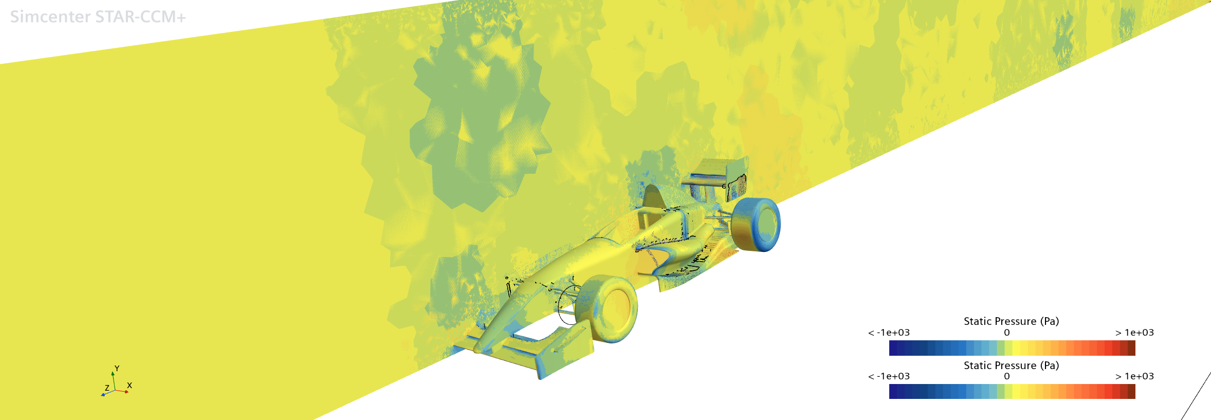
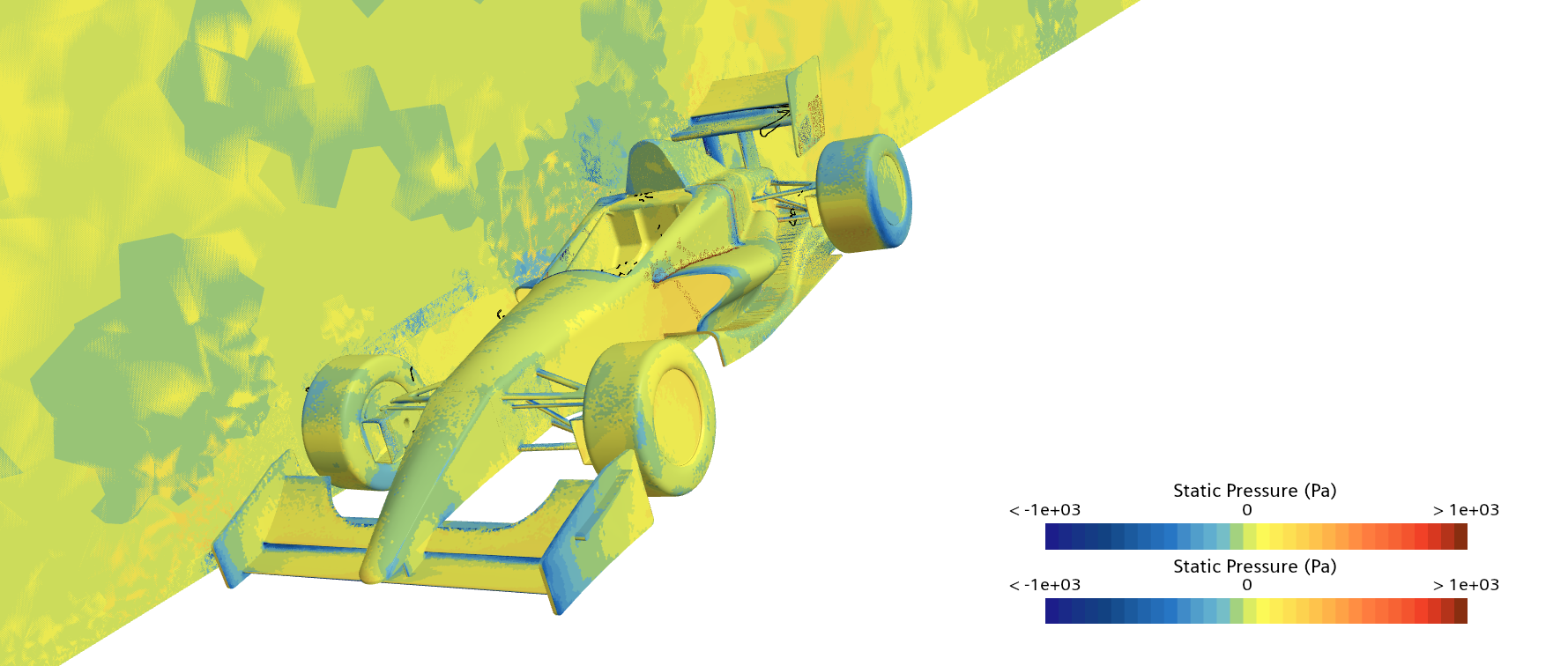
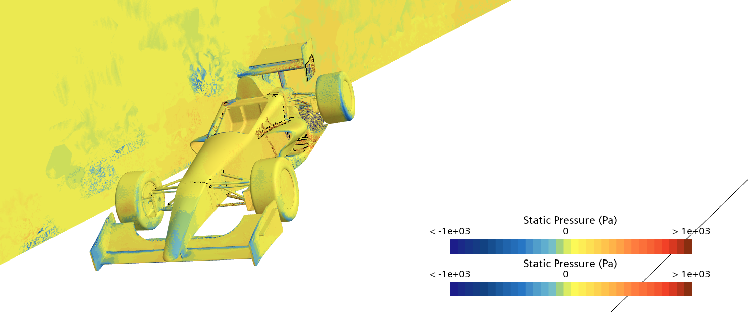
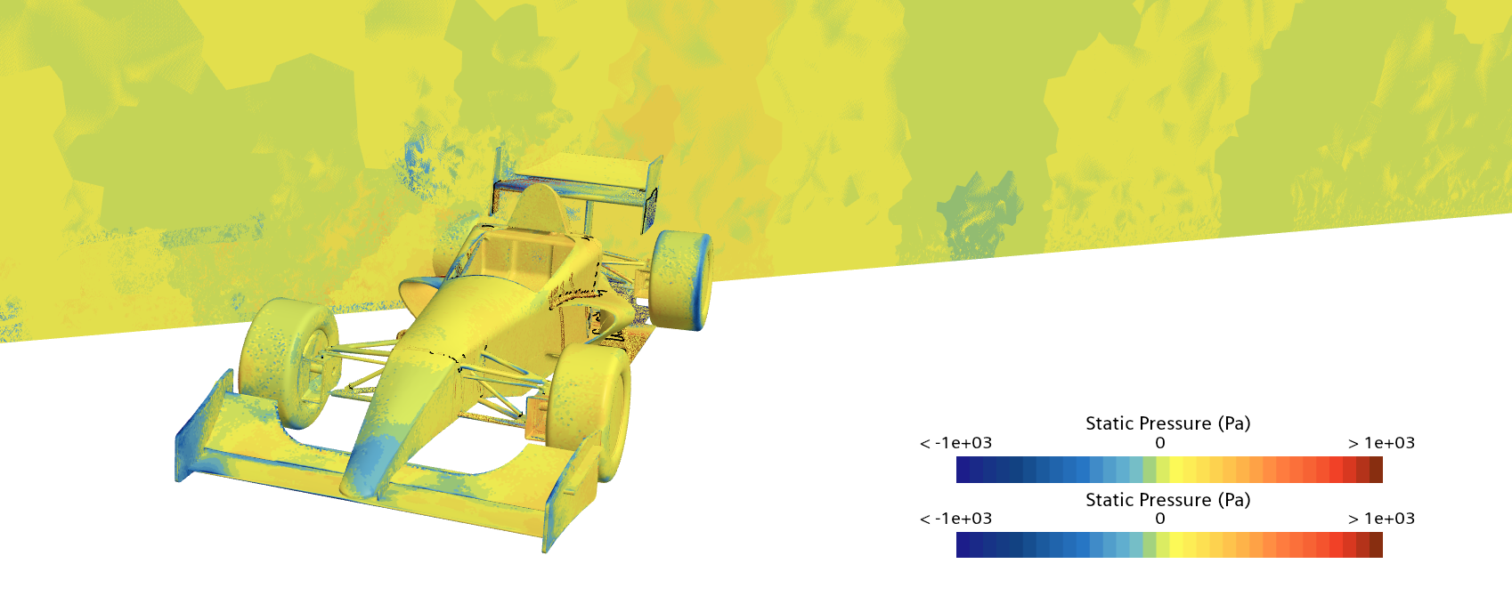
The scenes show static pressure relative to the simulation’s reference pressure. Blue marks lower pressure and red marks higher pressure on the displayed scale. Pa means pascals; 1e+03 means 1,000. The scale limits are −1,000 to +1,000 Pa; the end symbols mark values outside that range.
Select an angle to inspect the vehicle surfaces and the adjacent slice through the air. Each image opens at full size with its original scale bars.
0° yawStatic pressure
 View full size ↗
5° yawStatic pressure
 View full size ↗
15° yawStatic pressure
 View full size ↗
30° yawStatic pressure
 View full size ↗
45° yawStatic pressure
 View full size ↗
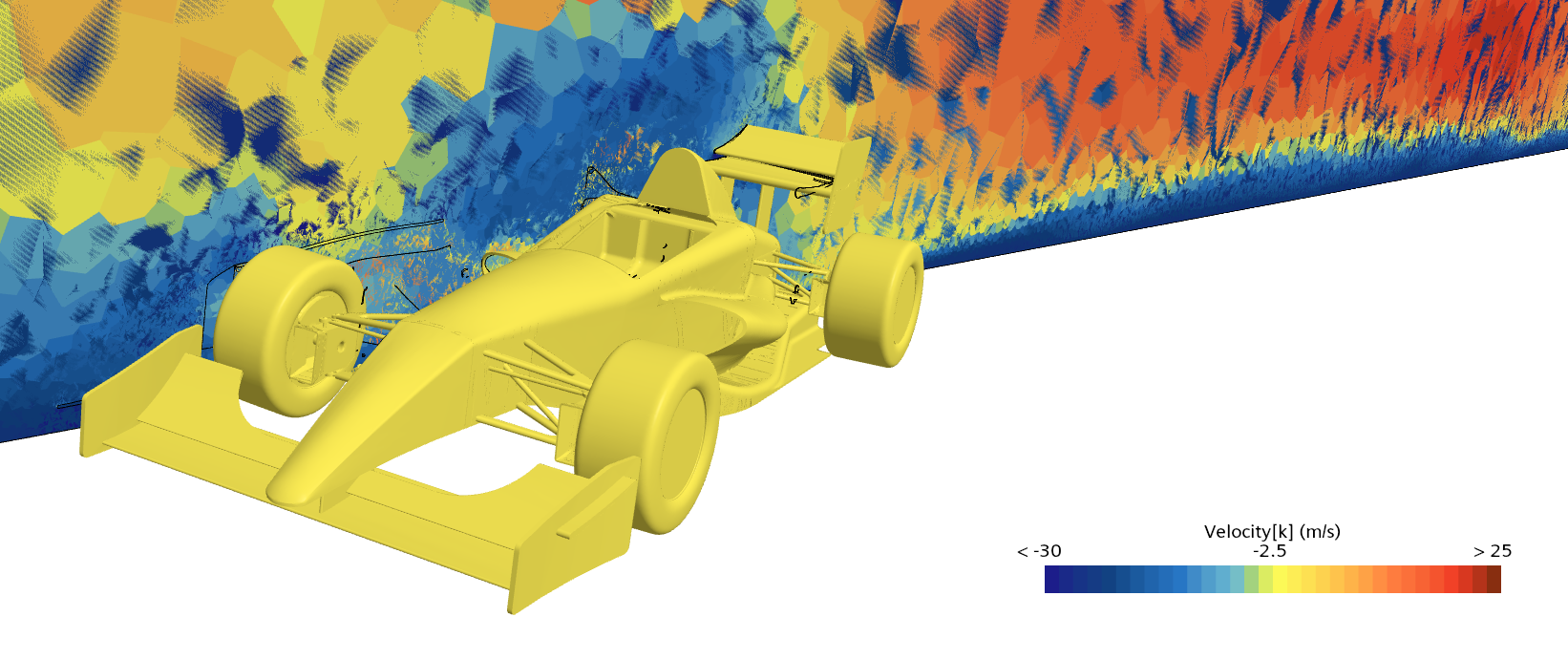
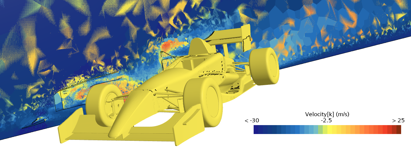
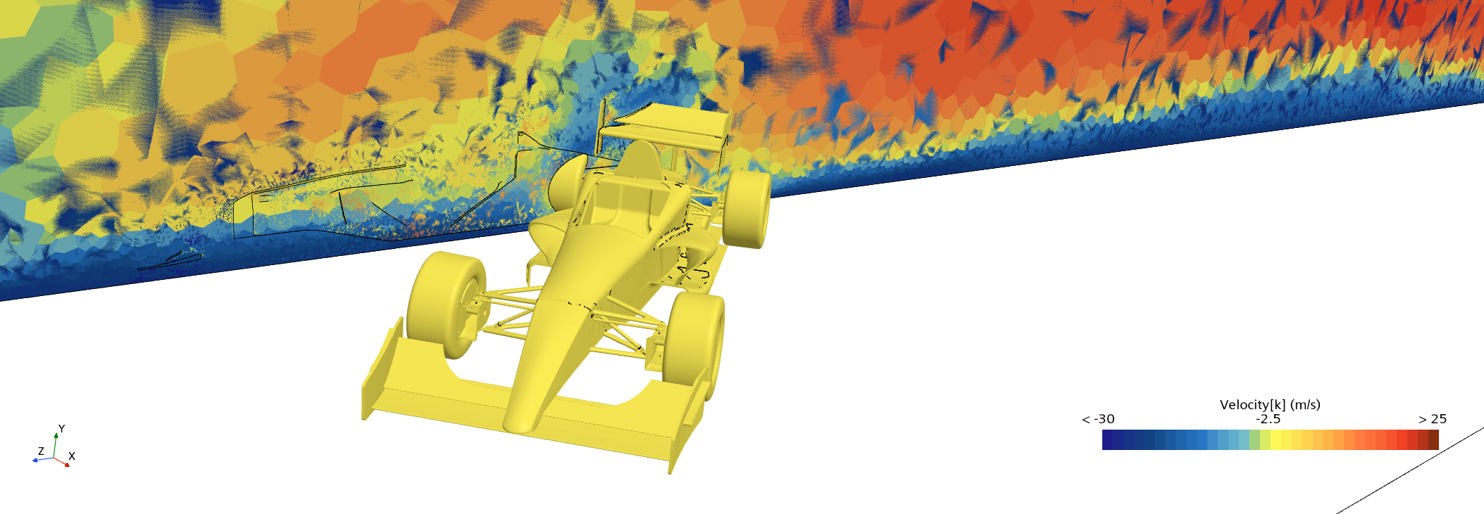
A component of the airflow velocity
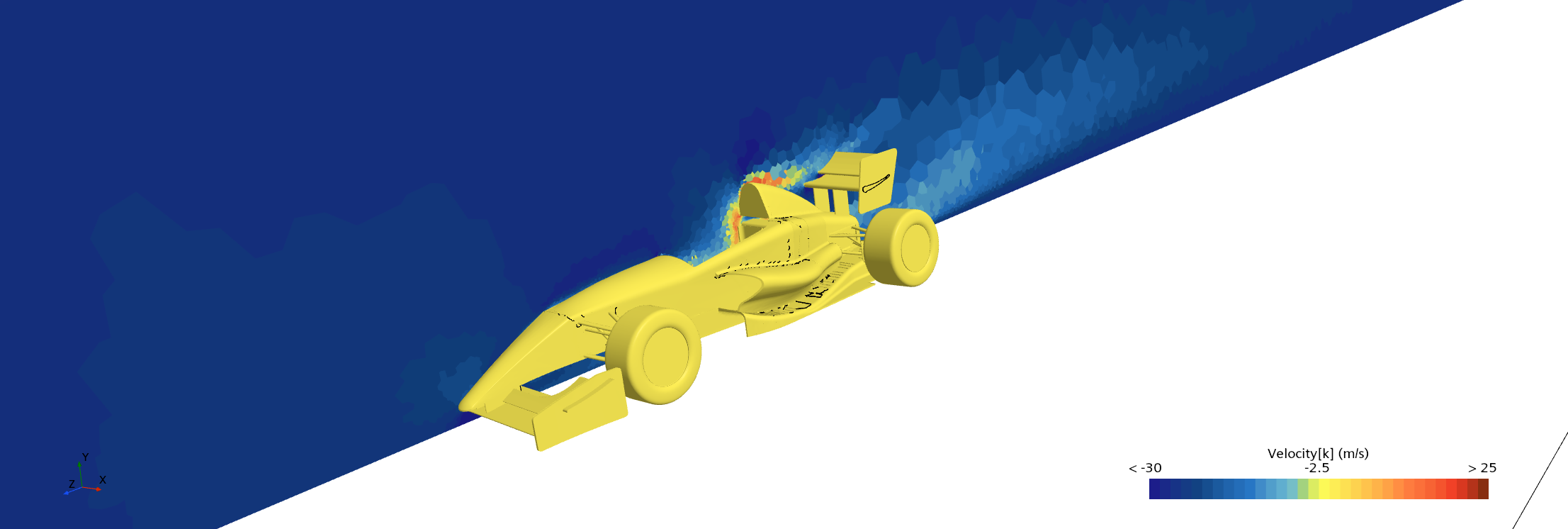
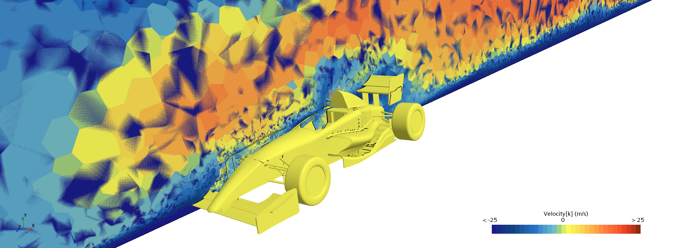
These scenes show Velocity[k], the signed Z component of velocity, in metres per second (m/s). They show movement along one coordinate direction, rather than total airspeed. Negative values indicate motion in the negative Z direction; they do not on their own prove reverse flow along the car.
0° yawSigned Z velocity
 View full size ↗
5° yawSigned Z velocity
 View full size ↗
15° yawSigned Z velocity
 View full size ↗
30° yawSigned Z velocity
 View full size ↗
45° yawSigned Z velocity
 View full size ↗
The colour scales and camera views must be checked before comparing scenes. Their spatial patterns do not measure fluctuations over time. Confirming separation or vortices requires further flow analysis; colours alone do not establish either mechanism.
How yaw affects vehicle performance
Maximum speed and drag power
More aerodynamic resistance leaves less power available for acceleration and can reduce maximum speed. The power needed to overcome that resistance is the resisting force along the direction of travel multiplied by vehicle speed.
In a crosswind, vehicle speed over the ground differs from airspeed relative to the car. The aerodynamic force must also be resolved into the direction of travel, including the contribution of side force. A low drag coefficient at yaw therefore cannot be converted directly into a higher maximum speed or lower engine power demand.
Acceleration and response from 80 to 120 km/h
At the same driving force, lower resistance leaves more force to accelerate the car. This can shorten an acceleration interval such as 80–120 km/h, often called an elasticity test. The gear and shift strategy must remain the same for a fair comparison.
However, a loss of downforce can reduce the tyre load available for traction. The result depends on whether the car is limited by engine power or tyre grip at that speed. These yaw cases do not provide a new set of acceleration or elasticity times.
Cornering and braking
Downforce adds load at the tyres without adding vehicle mass. A loss of that load can reduce cornering and braking capacity. The change in grip will depend on the tyres and how load is distributed; it does not equal the percentage change in downforce.
Total load is also only part of the picture. Different losses at the front and rear could change handling balance. We need axle loads or pitching moments to determine that shift, so these total coefficients cannot identify an understeer or oversteer response.
Directional stability
Yaw can create a side force and a yawing moment, a turning effect about the car’s vertical axis. Their magnitude and direction help determine how the vehicle responds to a disturbance.
A downforce loss alone does not prove instability. Establishing stability requires side forces, moments, tyre behaviour and the response over time. Those results are not supplied by this five-angle comparison.
Using yaw results in development
The cases indicate strong yaw sensitivity in this model, particularly in the lift coefficient between 0° and 5°. That step deserves closer checks and more test points before it is used as a design limit.
The simulations use a stationary floor and non-rotating wheels. These simplifications limit how closely the airflow represents a car on track. Force convergence, mesh sensitivity, reference areas and force directions also need to be established before the numerical differences support firm performance claims.
A useful next study would examine smaller positive and negative yaw angles, use moving ground and rotating wheels, and record front and rear loads, side force and yawing moment. It could then be connected to a vehicle model and checked against physical testing.
The development aim is to retain useful load and predictable balance as the airflow direction changes. The lowest drag coefficient at one angle cannot establish that outcome.
Model credit and special thanks
Special thanks to Dan Serban for creating the CAD model used in this study. His Formula-type single seater provides the geometry used for the yaw comparisons.
Serban, D. (2022) Formula-type single seater. GrabCAD Community [CAD File]. Available at: https://grabcad.com/library/formula-type-single-seater-1/details?folder_id=12079124 (Accessed: 21/10/2025).
Further reading on coefficient definitions and force directions: NASA Glenn Research Center, Drag Coefficient and Force Balance Coordinates.