
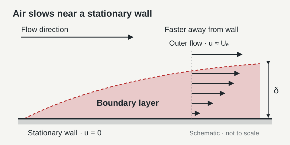
Air does not move at the same speed everywhere inside a wind tunnel. It slows near the floor, roof and side walls. These regions affect the flow reaching a test model, so the tunnel itself forms part of the aerodynamic experiment.
Our first two articles examined changes to a car’s shape and changes to the airflow direction. This article looks at the surrounding air volume. Using the Oxford Brookes University wind tunnel as an example, we can explain boundary layers and decide when computational fluid dynamics (CFD) should reproduce a physical tunnel.
What is a boundary layer?
Air has viscosity: it resists differences in motion between adjacent regions. At a solid surface, air takes the velocity of that surface. This is the no-slip condition. Next to a stationary wall, the air velocity is zero.
Farther from the wall, the air moves faster until it approaches the speed of the outer flow. The region containing this change is the boundary layer. Its edge is not a sharp surface. We commonly define its thickness at the position where the velocity reaches 99% of the local outer-flow value.
Boundary layers form on a car’s body, wings and floor, as well as on tunnel walls. They produce skin-friction drag and affect how the flow responds to pressure changes. If pressure rises sufficiently in the flow direction, the slower air near a surface can reverse and the flow can separate. This can change drag and downforce.
A boundary layer can be laminar, with relatively ordered motion, or turbulent, with fluctuating motion and stronger mixing. Under comparable flat-plate conditions, a turbulent layer generally grows faster and produces more skin friction. Its mixing can also help it remain attached against a rising pressure.
See NASA Glenn’s boundary layer explanation for the link between near-surface flow, friction and separation.
Three ways to describe the same layer
A single thickness cannot describe every effect of a velocity profile. Engineers use three related quantities, each with units of length.
- Boundary layer thickness, δ
- The distance from the wall to approximately 99% of the local outer-flow speed. It describes how far the velocity deficit extends.
- Displacement thickness, δ*
- The equivalent distance by which the wall would need to move into an ideal uniform flow to produce the same reduction in volume flow. It measures the effect of the slower air on the flow outside the layer.
- Momentum thickness, θ
- A measure of the momentum-flow deficit caused by the slower air. It helps relate boundary layer development to wall friction and pressure gradients.
These are three descriptions of one velocity profile. They are not three separate layers. In particular, δ* is much smaller than δ in the estimates below. Treating the entire boundary layer as a solid obstruction would exaggerate its effect: most of the air inside it is still moving.
MIT’s definitions of integral thickness give the mathematical form of displacement and momentum thickness.
The Oxford Brookes wind tunnel example
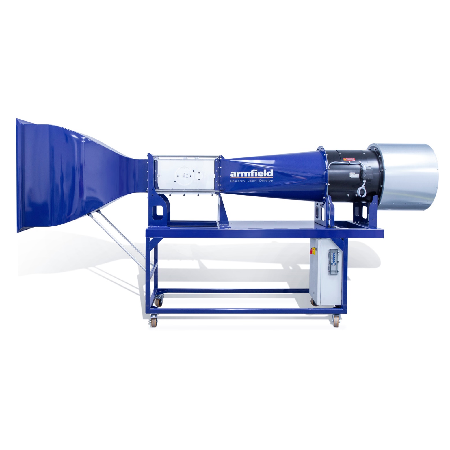
The Armfield tunnel considered here has a 310 × 310 mm working section, 660 mm long. We examine a nominal working-section speed of 40 m/s, with air at 20°C and 100 kPa. These are the conditions used for the calculations, rather than a measured velocity at every point.
 View full size ↗
Air is drawn from the room and discharged back into it, making this an open-circuit tunnel. The working section still has solid walls. Open circuit describes the air’s route through the facility; it does not mean that the model is in unrestricted open air.
The inlet honeycomb helps straighten the airflow. Together with suitable flow-conditioning components, it can reduce unwanted disturbances. Its presence does not prove that the wall boundary layers are turbulent. A relatively uniform core flow can exist alongside developing wall layers.
The dimensions and flow-straightener arrangement are described in Armfield’s C30 datasheet. NASA’s flow-conditioning experiments also show how honeycomb and screens can reduce tunnel turbulence.
Why the air accelerates through the inlet
The inlet contracts from a large opening into the smaller working section. At these low speeds, treating air density as approximately constant is a useful first approximation. The same volume flow must then pass through each cross-section, so the average speed rises as the area falls.
Volume flowQ = Uavg × A
For the working-section scenarioQ ≈ 40 × 0.310 × 0.310 = 3.84 m³/s
Here, Q is volume flow, A is cross-sectional area and Uavg is average velocity. For this initial calculation, the nominal 40 m/s is treated as the section average. A centreline probe reading would need a velocity-profile correction before it could give an exact volume flow.
The contraction profileDimensions along the tunnel
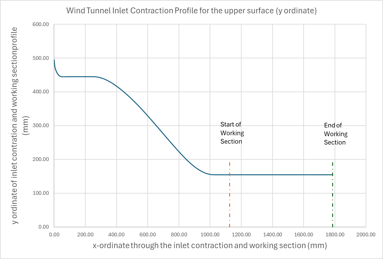 View full size ↗
Inside the contractionSectioned CAD view
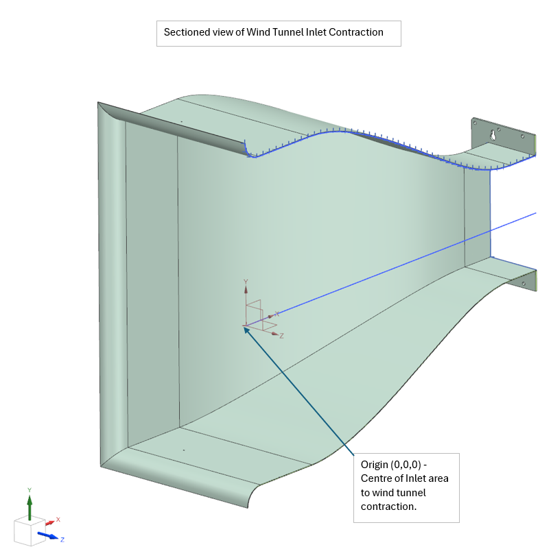 View full size ↗
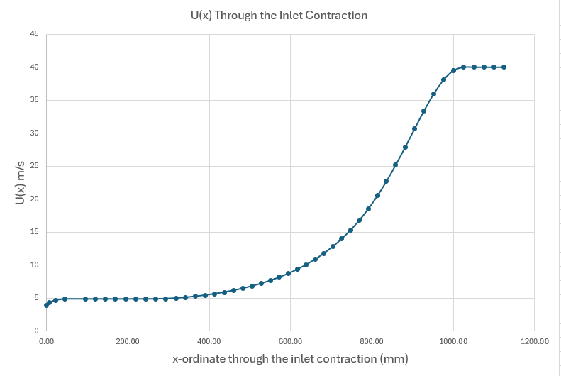 View full size ↗
The last distinction matters. The bulk velocity can reach 40 m/s while the velocity at a stationary wall remains zero. The contraction also changes the pressure gradient, so a wall layer carries the influence of the upstream flow into the working section.
What the thickness estimates can tell us
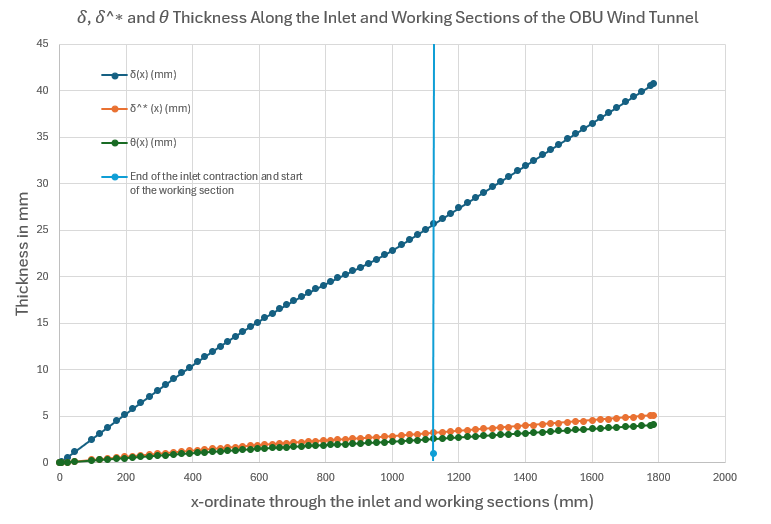
A simple turbulent-layer calculation gives the following development along one wall. It places δ at approximately 26 mm at the working-section entrance and 41 mm near its exit. The corresponding displacement thickness rises from about 3.2 to 5.1 mm, and momentum thickness from about 2.6 to 4.1 mm.
 View full size ↗
The plot illustrates why the wall region cannot be ignored. However, its numerical values are sensitive to the calculation method. A duct Reynolds number and a boundary layer Reynolds number use different length scales. They cannot be substituted directly into the same correlation.
For this square passage, the hydraulic diameter is 0.310 m. At 40 m/s, using a kinematic viscosity of approximately 1.5 × 10⁻⁵ m²/s gives a duct Reynolds number of about 8.3 × 10⁵. This remains constant through the uniform working section. A Reynolds number based on downstream distance continues to increase.
Check the estimate using a flat-plate reference
A common turbulent flat-plate correlation is δ ≈ 0.16x / Rex1/7, with Rex = Uex / ν. Here, x is distance from a defined leading edge, Ue is the outer-flow speed and ν is kinematic viscosity.
For a reference plate exposed to 40 m/s from its leading edge, with turbulent flow assumed from that edge, the distances corresponding to the tunnel stations give:
| Distance x | Rex | Thickness δ |
|---|---|---|
| 1.125 m | 3.00 × 10⁶ | 21.4 mm |
| 1.785 m | 4.76 × 10⁶ | 31.8 mm |
The difference from 26–41 mm shows the importance of the Reynolds-number definition. Neither calculation resolves the actual contraction, pressure gradient, initial wall profile or laminar-to-turbulent transition. Predicting the real thickness requires a suitable boundary layer calculation, resolved CFD or velocity measurements.
The correlation is described in Louisiana Tech’s flat-plate boundary layer notes.
Similarly, the familiar transition value near Re = 2,300 belongs to internal pipe-flow reasoning. It does not locate transition on these tunnel walls. Surface roughness, incoming disturbances and the pressure gradient also matter. A turbulent-layer assumption must therefore be identified as an assumption.
The working section is only about 2.1 hydraulic diameters long. A simple turbulent duct entrance-length estimate gives roughly 13 m, much longer than 0.66 m. That is a scale comparison, not an exact prediction for this contraction-fed passage. We should not assume that its velocity profile is fully developed, meaning unchanged in shape along the duct.
Why a few millimetres can affect a test
Boundary layers develop on all four working-section walls. Their velocity deficits reduce the passage’s effective flow area. For a fixed volume flow, the faster core must carry the difference. Adding a model introduces further blockage and changes the surrounding pressure field.
Consider an illustrative displacement thickness of 5 mm on each wall. A simple equivalent-area estimate gives (310 − 2 × 5)² = 90,000 mm², compared with the physical 96,100 mm². That is about 6.3% less effective area.
Under the same-volume-flow assumption, the core speed would be about 6.8% higher than the bulk speed. Dynamic pressure depends on speed squared, so it would be about 14% higher. This is an illustration of the displacement effect; it is not a measured tunnel correction or a prediction of a 14% force error.
The actual result depends on the velocity profile, corners, model size, reference-speed location and how the tunnel is controlled. Walls can also restrict the flow displaced by the model and alter its wake. These effects help explain why the same wing can give different results in a confined tunnel and in open air.
Choosing the right environment for CFD
In vehicle CFD, we often hold the car fixed and move the air past it. This avoids moving the complete car through a very large mesh. It is a choice of reference frame: it can represent either a wind tunnel or a car travelling through open air.
A fixed computational domain does not automatically represent a wind tunnel. The domain is the finite volume in which the flow is calculated. Its dimensions and boundary conditions determine what environment it represents.
When the aim is to match a wind tunnel
To compare CFD with uncorrected tunnel measurements, we should reproduce the relevant test conditions. That includes the working-section geometry, stationary no-slip walls, model location, support hardware and the incoming velocity and turbulence profiles. We also need consistent reference speeds, air properties and force definitions.
The inlet can include the contraction, allowing the wall layers to develop through it. Alternatively, a shorter model can start with measured or otherwise justified inlet profiles. A uniform inlet immediately ahead of the model can miss the wall layer already present in the physical tunnel.
CFD then helps separate the model’s response from the facility’s influence. NASA’s comparison of tunnel and free-air simulations demonstrates why representing the tunnel environment can be necessary for a meaningful experimental comparison.
When the aim is to represent the car on track
For open-air vehicle development, the outer boundaries should be far enough away that they have little effect on the result. Suitable open, far-field or slip/symmetry conditions can be used according to the solver and flow direction. Increasing the domain size is one way to check the remaining boundary influence.
In the fixed-car frame, the road normally moves with the incoming stream and the wheels rotate at the corresponding speed. A moving ground plane avoids introducing the stationary-floor boundary layer of a simple fixed-floor tunnel. At yaw, road motion must remain consistent with vehicle motion, while the air direction also accounts for wind.
Both approaches use a bounded computational volume. The choice is whether its boundaries reproduce a physical facility or approximate the surroundings of the vehicle. A tunnel model is useful for experimental validation; an open-air model is useful for the intended track condition.
What this changes in aerodynamic development
The Oxford Brookes example shows two changes occurring together: the contraction accelerates the bulk flow, while the walls create velocity deficits close to their surfaces. A single tunnel-speed value cannot describe both.
Before comparing a CFD result with a test, we need to know where speed was measured, which wall and ground conditions were used, and whether the experimental data include tunnel corrections. Otherwise, a difference caused by the environment can be mistaken for a geometry or turbulence-model error.
Mesh refinement near the walls and a suitable near-wall treatment are also necessary. The calculation must capture the velocity gradients, and its forces must be sufficiently converged. Reproducing the tunnel shape alone does not establish accuracy.
Once the tunnel comparison is understood, a separate open-air calculation can investigate the intended operating condition. This connects the experiment to vehicle development while keeping the assumptions of each result clear.
Figures and further reading
Equipment image: Armfield, C30 Computer Controlled Wind Tunnel. Inlet profile and sectioned CAD: Bell, D. (2025), Armfield Wind Tunnel Inlet Contraction and Working Section Profile, Oxford Brookes University. The velocity and thickness plots are calculations for the stated example; the opening schematic is explanatory.
The linked NASA, MIT and Louisiana Tech resources explain the underlying flow physics and modelling methods. The initial thickness curve is retained with its calculation limits stated beside it. No measured boundary layer profile or validated tunnel-force correction is claimed.