
A CFD result becomes more useful when we know how closely it represents a physical test. A wind tunnel gives us measurements to make that check. Comparing the two helps us find where a simulation predicts the right behaviour and where its limits could affect a design decision.
Our earlier articles explained how geometry, yaw, boundary layers and body shape change aerodynamic performance. Here, we use a NACA 0015 wing in the Oxford Brookes University wind tunnel to examine the next question: how much confidence should we place in the prediction?
Start with the same wing and conditions
The NACA 0015 is a symmetric aerofoil. Its maximum thickness is 15% of its chord, the distance from the leading edge to the trailing edge. The example uses a nominal 150 mm chord, with CFD at 25 m/s. The recorded tunnel speeds in the force tests range from 24.64 to 25.34 m/s.
The wing was tested over angles from 0° to 18° in 2° steps. Positive angle labels in the force dataset describe increasing downforce, so they use the opposite sign to the usual convention for an aerofoil producing upward lift. We retain those test labels here. The angle origin and direction must be checked before two datasets are compared.
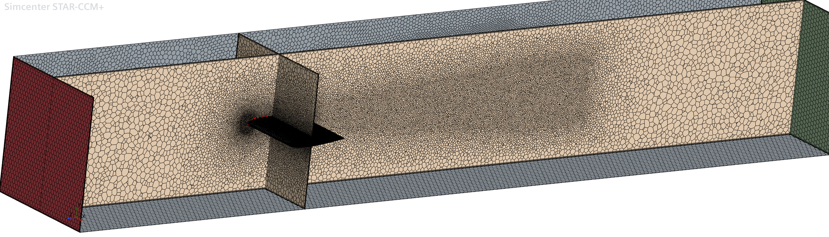
The CFD model includes the tunnel walls. As the boundary layer article explained, those walls affect the flow reaching the model. A useful comparison also needs matched wing dimensions, position, surface condition, inlet flow and mounting conditions. Matching speed alone is insufficient when model size or air properties differ: the Reynolds number must also be considered.
Small speed differences matter because aerodynamic force scales approximately with speed squared when the flow regime is unchanged. Coefficients help remove that direct scale effect. They do not remove changes caused by Reynolds number, transition or separation.
Compare pressure at the same locations
A pressure tap is a small opening in the wing surface connected to a pressure measurement system. It samples local surface pressure. Ten taps were used here, with matching CFD probe locations. Their chordwise positions run from 0 to 130.7 mm behind the leading edge.
See the ten pressure tap positions
| Tap | Position (mm) |
|---|---|
| 1 | 0.0 |
| 2 | 7.4 |
| 3 | 14.2 |
| 4 | 22.6 |
| 5 | 33.8 |
| 6 | 47.0 |
| 7 | 63.2 |
| 8 | 82.3 |
| 9 | 105.4 |
| 10 | 130.7 |
We convert pressure into the dimensionless pressure coefficient, Cp. This places both methods on a common scale:
Pressure coefficientCp = (p − p∞) / (½ρU∞²)
Here, p is local surface pressure, p∞ is the reference static pressure, ρ is air density and U∞ is reference air speed. A negative Cp means pressure below the reference value. The CFD reference pressure was sampled upstream of the wing. Both methods need consistent pressure references and units.
The difference between the pressure distributions on the two surfaces helps produce the wing’s load. The suction side is the lower-pressure surface; the pressure side is the higher-pressure surface. These names remain useful when a wing is inverted to produce downforce.
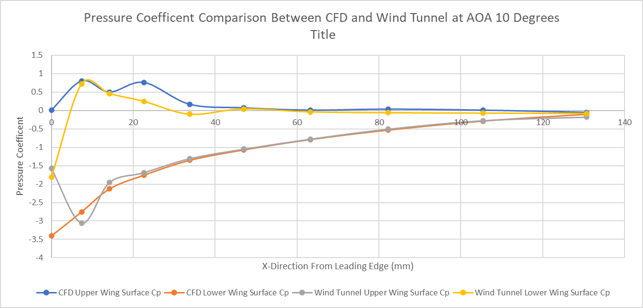
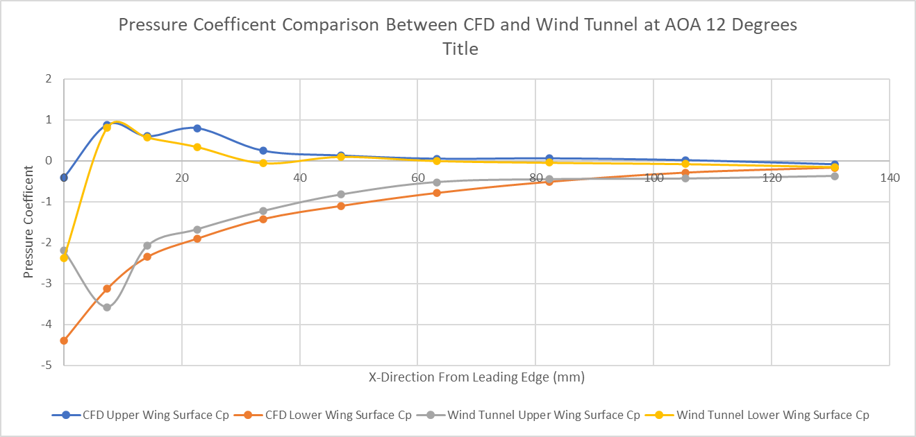
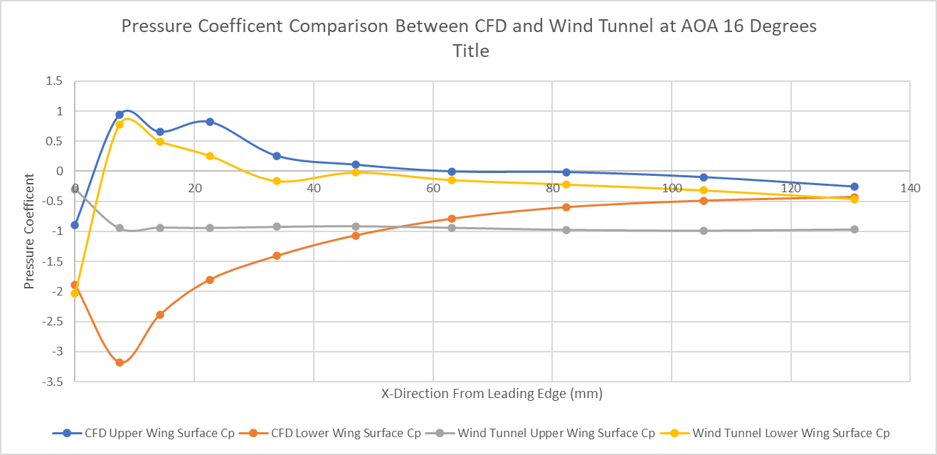
Reading the original plots: the recorded upper/lower labels use opposite orientations between the two methods. In the nonzero-angle original plots below, compare orange CFD with grey tunnel data for the suction branch, and blue CFD with yellow tunnel data for the pressure branch. Negative Cp is plotted downwards. Smooth connecting lines are visual guides, not extra measurements.
Only one surface carried the experimental taps. Opposite-angle runs were used to infer the other surface, assuming symmetric flow conditions as well as a symmetric profile. This is a useful approximation, but it does not replace simultaneous measurements on both surfaces. Formal validation would also require confirmation of the physical angle and surface mapping.
What the pressure comparison shows
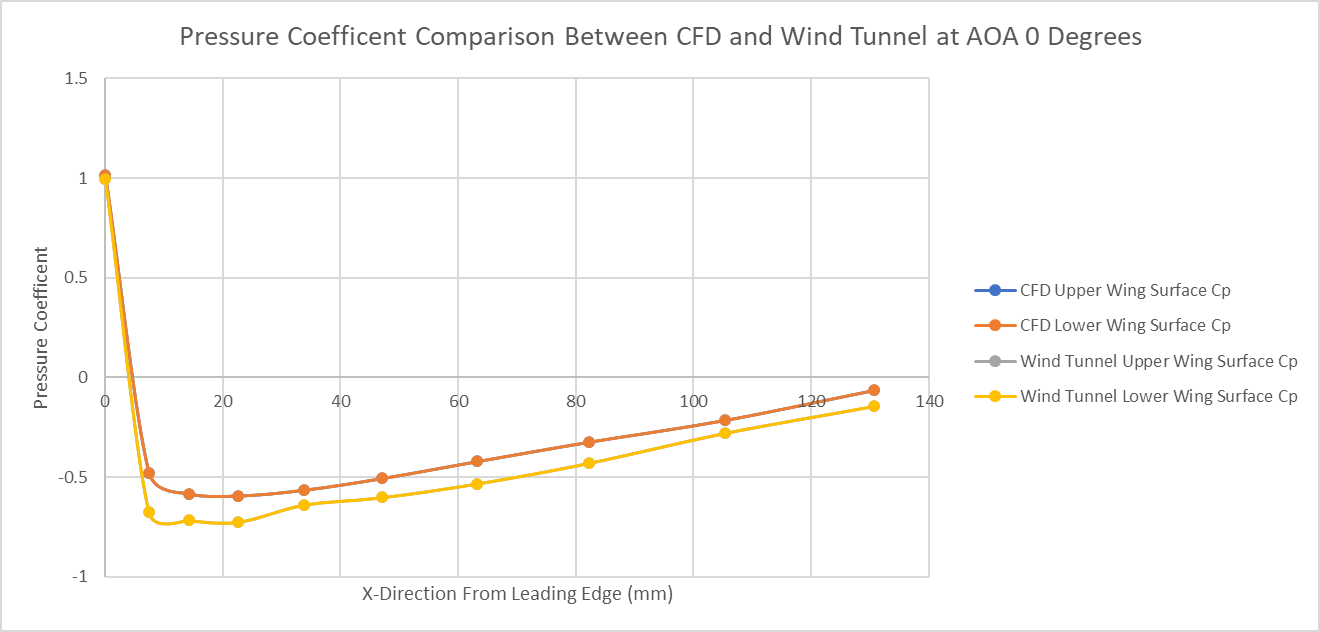
At 0°, both methods show pressure near Cp = 1 at the nose, followed by suction and a gradual return towards the reference pressure. The overall shape agrees, but the values differ. At tap 2, the tunnel gives −0.677 and CFD gives −0.478. CFD therefore predicts less suction at this location.
 View full size ↗
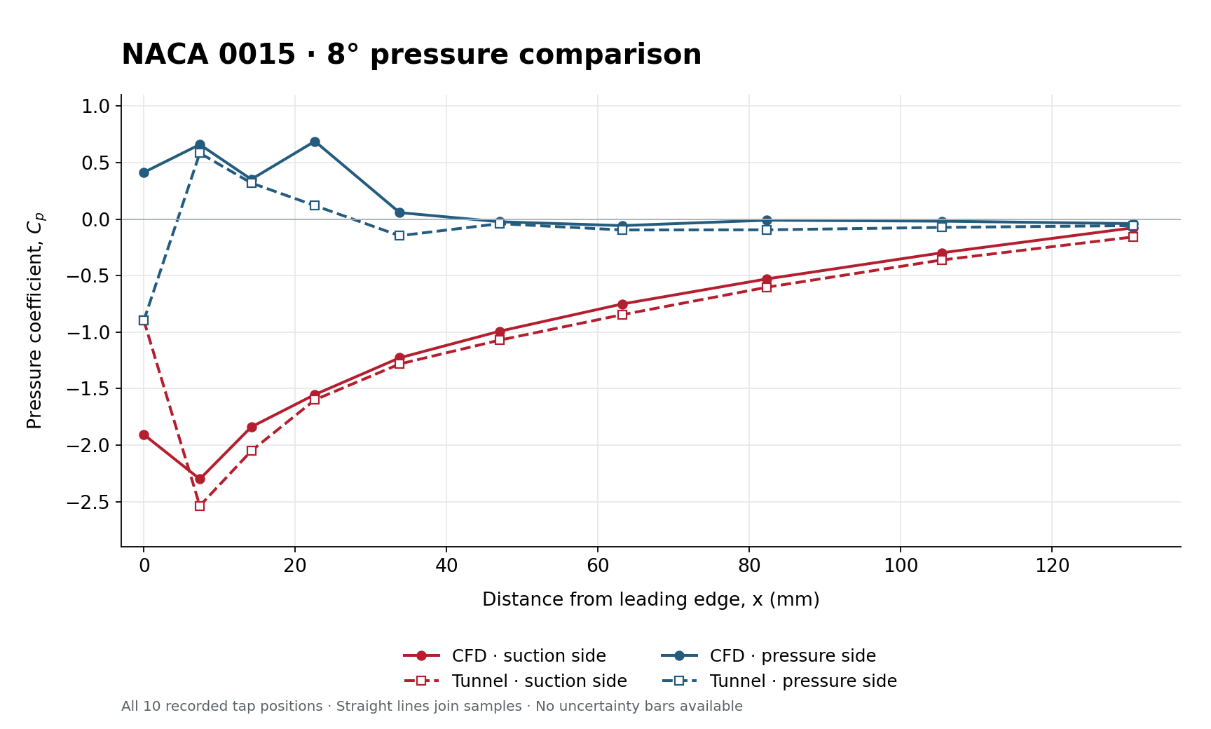
At 8°, both methods show a suction peak near the front and pressure recovery towards the rear. From tap 2 rearwards, the suction branches follow a similar trend. They still differ at the nose and on parts of the pressure side. For example, at x = 22.6 mm, pressure-side Cp is about +0.688 in CFD and +0.119 in the tunnel.
 View full size ↗
At 10° and 12°, the leading-edge differences become particularly important. At 12°, the first suction-side sample is about −4.40 in CFD and −2.20 in the tunnel. Yet at tap 2, the tunnel has the more negative value. The difference is therefore in the pressure distribution’s shape, not a constant offset that we can remove from every reading.
10° pressure distributionInspect the leading edge
 View full size ↗
12° pressure distributionA larger local difference
 View full size ↗
At 16°, the disagreement changes character. The tunnel suction-side readings are nearly flat, around Cp = −0.9 to −1.0 from tap 2 onwards. CFD retains a strong forward suction peak and a recovery towards the trailing edge. The measured plateau is consistent with extensive separated flow. The two methods are no longer describing the same pressure distribution.
 View full size ↗
| Angle | Tunnel | CFD | Absolute difference |
|---|---|---|---|
| 0° | −0.68 | −0.48 | 0.20 |
| 8° | −2.54 | −2.30 | 0.24 |
| 10° | −3.05 | −2.75 | 0.30 |
| 12° | −3.57 | −3.12 | 0.45 |
| 16° | −0.95 | −3.18 | 2.23 |
The difference at this one location increases substantially at 16°. It is not an error measure for the whole wing. A complete assessment must include the other taps, both surfaces and the forces.
Check total forces as well as local pressure
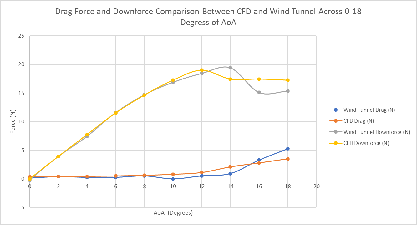
The force comparison initially looks encouraging. At 8°, the tunnel measured 14.67 N downforce and CFD predicted 14.61 N, a difference of about 0.4%. This close force agreement exists alongside the local pressure differences above. Errors in different parts of a surface can partly cancel when their contributions are added together.
 View full size ↗
| Angle | Tunnel (N) | CFD (N) | Difference |
|---|---|---|---|
| 8° | 14.67 | 14.61 | −0.4% |
| 12° | 18.42 | 18.97 | +3.0% |
| 14° | 19.41 | 17.42 | −10.2% |
| 16° | 15.09 | 17.43 | +15.5% |
| 18° | 15.33 | 17.22 | +12.3% |
The highest sampled downforce occurs at 14° in the tunnel and 12° in CFD. By 16°, CFD predicts 2.33 N more downforce than the tunnel. Drag also differs: at 18°, the measured value is 5.27 N, compared with 3.49 N in CFD. The high-angle performance is therefore less favourable in the experiment than those CFD values suggest.
The pressure and force measurements came from separate experimental sets. They provide related evidence, but they cannot be treated as a simultaneous pressure-to-force check. The recorded zero drag at 10° also needs investigation; it does not establish that the wing produced no drag.
Why the results can differ
As angle increases, flow separation makes the problem harder to represent. CFD predictions depend on the mesh, turbulence treatment, near-wall treatment and whether the calculation represents changes with time. A converged force value does not, by itself, prove that the physical flow is correct.
The numerical mesh used local refinement near the leading and trailing edges and in the wake, with a 3 mm base size. The near-wall setup targeted y+ around 1, using a nominal 0.02 mm first-layer height and five prism layers. This dimensionless wall distance helps assess near-wall resolution. A target setting must still be checked in the completed solution.
Later baseline mesh adjustments changed the recorded forces by about 0.5% or less. However, these checks were not repeated across the full angle range. They do not establish the same numerical accuracy near stall. A comparison of y+ targets of 1 and 50 also showed that the pressure and wall-shear distributions depend on near-wall treatment. A smaller y+ alone cannot guarantee an accurate separation prediction.
The experiment has limits too. Wing oscillation was observed during high-angle force testing. Movement changes the angle seen by the flow and can affect measured loads. Sparse taps can miss a narrow pressure peak, while tubing, reference-pressure errors and angle-setting errors can affect readings. Opposite-angle reconstruction adds another assumption. The leading-edge differences also require a check that each CFD probe remained at the intended surface location as the wing rotated.
The supplied comparisons do not include repeatability ranges or quantified uncertainty bars. We can identify the differences, but we cannot assign all of them to CFD or declare an exact validation tolerance. The high-angle data remain useful evidence that the response needs further investigation.
What each method does well
| Task | CFD | Wind tunnel |
|---|---|---|
| Compare designs | Geometry can be changed without manufacturing each part. Detailed cases can still require substantial setup and computing time. | Measures physical hardware, but each model change needs manufacture, installation and tunnel time. |
| Inspect the flow | Provides pressure, velocity and other calculated fields throughout the domain. Their accuracy depends on the numerical model. | Provides physical measurements. Spatial coverage depends on taps, probes or optical equipment and their access. |
| Study separation | Can help locate and explain separated regions, but predictions can be sensitive to modelling choices and resolution. | Exposes the physical response, including fluctuations, if the instruments and sampling method capture it. |
| Represent the car | Can model full-scale geometry and controlled conditions, with assumptions about detail and motion. | Includes real surfaces and deformation, but scale, supports, tunnel walls and ground simulation can affect transfer to the track. |
In this example, CFD gives us the pressure field between the ten taps. The tunnel tests whether that predicted field is plausible at measured locations. Each method helps expose limits in the other.
Why correlation matters in motorsport
In motorsport, correlation means checking whether simulation, tunnel and track results agree closely enough to support the intended decision. It includes absolute loads, local flow behaviour and the change caused by an upgrade. Two curves can follow the same trend while remaining too far apart to guide a wing setting.
The NACA 0015 example makes that distinction clear. Selecting an angle from the predicted peak alone would give a different answer from selecting it from the measured peak. Transferred to a rear wing, an overprediction of high-angle load could affect the expected front-to-rear balance. Underpredicted drag could also overstate the performance benefit.
A useful comparison follows a controlled sequence:
- Match the case. Check geometry, angle, speed, density, Reynolds number, pressure references and relevant tunnel conditions.
- Check numerical sensitivity. Examine force histories, conservation and mesh effects at representative conditions, including near separation.
- Check the measurement. Calibrate instruments, verify angle settings, repeat tests and quantify uncertainty. Measure both surfaces directly where possible.
- Compare local and total results. Use pressure distributions alongside forces and moments. Investigate differences before changing model settings.
- Test further conditions. Use independent cases to check whether an improvement holds beyond the case used to adjust the model.
Matching an existing measurement by adjusting a model is calibration. Confidence increases when the adjusted model also predicts cases that were not used for that adjustment. NASA’s validation guidance likewise ties validation to a defined range of applications and requires experimental uncertainty to be considered.
For a complete race car, that range includes changes in ride height, pitch, yaw and wheel motion. Tunnel correlation supports the simulation under the tested conditions. Track measurements then check whether the result transfers to the operating car. A small predicted gain must be assessed against the uncertainty in that comparison before it supports a development decision.
From a wing test to a design decision
The NACA 0015 comparison shows useful agreement in parts of the lower-angle response, but clear local differences and a substantial loss of agreement at high angle. The close downforce result at 8° cannot establish accuracy across the whole operating range.
CFD helps us explore changes and understand the flow. Wind tunnel measurements test those predictions against physical behaviour. Correlation connects the two, so that a promising aerodynamic change can be judged on evidence before it is used on a race car.
Data and further reading
The numerical example uses the Oxford Brookes NACA 0015 pressure-tap and force datasets with corresponding STAR-CCM+ calculations. Pressure readings use experimental set 3; force readings use set 4. Six original mesh and comparison figures are retained. The 8° pressure chart is replotted from the tabulated values and positions. Differences are calculated from the unrounded values; no uncertainty bounds have been inferred.
NASA Glenn — Verification assessment explains checks on numerical implementation and calculation error. NASA Glenn — Examining spatial convergence describes how systematic grid studies assess discretisation error. NASA Glenn — Validation assessment explains comparison with experiments and the role of uncertainty.